Introduction

It's common for a machine learning model to not perform as well as expected when it's first trained. Deciding how to improve the performance of the model can be a difficult task, but understanding the bias and variance of a learning algorithm can give you a good idea of what to try next.

In this article, we'll take a look at what bias and variance mean in the context of machine learning and how they can be used to guide the development of a model. We'll use an example from linear regression to illustrate the concepts of bias and variance, and show how they can be used to diagnose and improve the performance of a model.

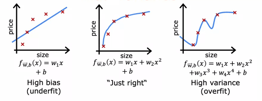
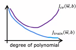
The example we'll use is a dataset of a single feature x, where we're trying to fit a straight line to the data. If we fit a straight line to the data, it doesn't do a very good job, and we say that the algorithm has high bias or that it underfits the dataset. If we fit a fourth-order polynomial, the algorithm has high-variance or it overfits the dataset. In the middle if we fit a quadratic polynomial, it looks pretty good. This is the "just right" model.

When you have more features, it's not as easy to visualize whether the model is doing well. Instead, a more systematic way to diagnose whether the algorithm has high bias or high variance is to look at the performance of the algorithm on the training set and on the cross-validation set.

To do this, we compute the training error, J_train, which is how well the algorithm does on the training set, and the cross-validation error, J_cv, which is how well the algorithm does on examples it has not previously seen.

• An algorithm with high bias, or underfitting, will have A high J_train and a high J_cv.
• An algorithm with high variance, or overfitting, will have a low J_train and a high J_cv.
• A good model, or one that is "just right," will have a low J_train and a low J_cv.

To summarize, when the degree of the polynomial is 1:

• J_train is high and J_cv is high, indicating high bias. (underfit)

When the degree of the polynomial is 4:

• J_train is low but J_cv is high, indicating high variance. (overfit)

When the degree of the polynomial is 2 :

• both J_train and J_cv are low, indicating a good model.

In conclusion, understanding the bias and variance of a machine learning algorithm can be a powerful tool in the development of a model. By looking at the performance of the algorithm on the training set and on the cross-validation set, you can diagnose whether the algorithm has high bias or high variance and take the appropriate steps to improve the performance of the model.

Regularization

Regularization is a technique used to prevent overfitting in machine learning models. It does this by adding a penalty term to the cost function that the model is trying to optimize. The regularization parameter, Lambda, controls the trade-off between keeping the model's parameters small and fitting the training data well. In this article, we will explore how the choice of Lambda affects the bias and variance of a fourth-order polynomial regression model, and how to choose a good value of Lambda using cross-validation.

When Lambda is set to a large value, the model is highly motivated to keep the parameters small, resulting in a model that is underfitting the training data. This can be seen in the example:

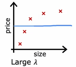
• where Lambda is set to 10,000
• where the model is roughly a constant value
• has high bias and a large J_train error.

On the other hand, when Lambda is set to a small value, such as zero, there is no regularization, and the model is overfitting the data. This can be seen in the example:

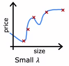
• where Lambda is set to 0
• where the model is a wiggly curve
• has high variance and a large J_cv error.

The goal is to find an intermediate value of Lambda that results in a model that fits the data well, with a small J_train and J_cv error. One way to do this is by using cross-validation. The process involves trying out a range of possible values for Lambda, fitting the parameters using those different regularization parameters, and then evaluating the performance on the cross-validation set. The value of Lambda that results in the lowest J_cv error is chosen as the optimal value.

In the example provided, after trying different values of Lambda, it was found that :

• J_cv of W5, B5 had the lowest value, and thus this value for Lambda was chosen.
• To estimate the generalization error, the test set error, J_tests of W5, B5, is reported.

The figure provided also illustrates how the training error and cross-validation error vary as a function of the parameter Lambda. At the extreme of Lambda equals zero, the model has a high variance and J_train is small while J_cv is large, as the model does well on the training data but not on the cross-validation set.

Regularization is an important technique in machine learning to prevent overfitting and the regularization parameter Lambda controls the trade-off between keeping the model's parameters small and fitting the training data well. The choice of Lambda can affect the bias and variance of the model and overall performance. Cross-validation can be used to choose a good value of Lambda by trying out a range of possible values and evaluating the performance on the cross-validation set.

Level of performance

Speech recognition is a crucial technology that enables users to search the web on their mobile phones by speaking, rather than typing on tiny keyboards. The job of speech recognition algorithms is to transcribe audio inputs, such as "What is today's weather?" or "Coffee shops near me," into text.

However, even with the best algorithms, speech recognition is not a perfect process. In this section, we will explore how to measure the performance of a speech recognition algorithm and determine if it has high bias or high variance.

One way to measure the performance of a speech recognition algorithm is to calculate the training error, which is the percentage of audio clips in the training set that the algorithm does not transcribe correctly in its entirety. For example: If the training error for a particular dataset is 10.8%, this means that the algorithm transcribes the audio perfectly for 89.2% of the training set, but makes some mistake in 10.8% of the training set.

Another way to measure the performance of the algorithm is to calculate the cross-validation error, which is the percentage of audio clips in a separate cross-validation set that the algorithm does not transcribe correctly in its entirety. For example: If the cross-validation error for a particular dataset is 14.8%, this means that the algorithm transcribes the audio correctly for 85.2% of the cross-validation set, but makes mistakes in 14.8% of the cross-validation set.

At first glance, it may seem that a training error of 10.8% and a cross-validation error of 14.8% indicate that the algorithm has high bias. However, it is also important to consider the human level of performance when analyzing speech recognition. In other words, how well can even humans transcribe speech accurately from an audio clips with wrong quality ? For example: If you measure how well fluent speakers can transcribe audio clips, and you find that human level performance achieves 10.6% error, it becomes clear that it is difficult to expect a learning algorithm to do much better.

Therefore, to judge if the training error is high, it turns out to be more useful to see if the training error is much higher than a human level of performance. In this example, the algorithm's training error is just 0.2% worse than humans, which is not a significant difference. However, the gap between the training error and cross-validation error is much larger, at 4%. This suggests that the algorithm has more of a variance problem than a bias problem.

When judging the performance of a speech recognition algorithm, it is important to establish a baseline level of performance. This can be done by measuring human level performance, comparing to a competing algorithm, or guessing based on prior experience. Once a baseline level of performance has been established, the key quantities to measure are the difference between the training error and the baseline level, and the gap between the training error and cross-validation error. If the first difference is large, the algorithm has high bias, and if the second gap is high, the algorithm has high variance.

Learning curve

The learning curves for a model that fits a second-order polynomial quadratic function can be plotted in order to analyze the performance of the model.

The figure will have the horizontal axis as the training set size or the number of examples, and the vertical axis will be the error, which can be the cross-validation error (J_cv) or the training error (J_train). When plotting J_cv, it is expected that as the training set size increases, the model will learn better and the cross-validation error will decrease.

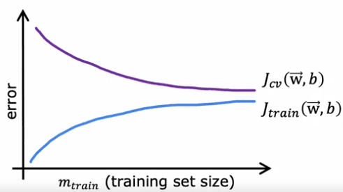
However, when plotting J_train, it is observed that as the training set size increases, the training error actually increases. This is because with a small number of training examples, it is relatively easy to achieve zero or very small training error, but as the training set size increases, it becomes harder for the quadratic function to fit all the training examples perfectly. Additionally, the cross-validation error is typically higher than the training error because the model is fitted to the training set, and so it is expected to perform better on the training set than on the validation set.

When comparing a model with high bias (underfitting) to one with high variance (overfitting), the learning curves will also differ:

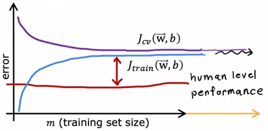
In the case of high bias, the training error will increase and then plateau as the training set size increases. This is because the model is too simple and so, even with more training examples, there is not much that can change. Similarly, the cross-validation error will decrease and then plateau.

In contrast, in the case of high variance, the training error will decrease while the cross-validation error will increase as the training set size increases.

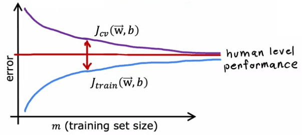
Analyzing learning curves can give insight into the performance of a model, and whether it is underfitting or overfitting. Additionally, it can be seen that as the training set size increases, it becomes harder for the model to achieve zero training error, and the gap between training and validation error will be an indicator of the model's bias-variance trade-off.

Decision

The training and cross-validation errors, Jtrain and Jcv, can give us a sense of whether our learning algorithm has high bias or high variance. In this article, we'll take a look at an example of regularized linear regression for predicting housing prices and explore how we can use this information to improve the performance of our algorithm.

When our algorithm has high bias, it means that it's not doing well even on the training set. In this case, the main ways to fix this problem are to get more training data or to add additional features. On the other hand, when our algorithm has high variance, it means that it's overfitting to a very small training set. To fix this problem, we can try to get more training examples or simplify our model by using a smaller set of features or increasing the regularization parameter Lambda.

Let's take a look at the example of regularized linear regression for predicting housing prices. In this case, we've implemented the algorithm but it's making large errors in predictions. To improve the performance of our algorithm, we have several options such as :

• getting more training examples
• trying a smaller set of features
• adding additional features
• adding polynomial features
• decreasing Lambda
• increasing Lambda.

The first option, getting more training examples, helps to fix a high variance problem. If our algorithm has high bias, then getting more training data by itself probably won't help that much. However, if our algorithm has high variance, then getting more training examples will help a lot.

Trying a smaller set of features can also help fix a high variance problem. Sometimes, if our learning algorithm has too many features, it gives the algorithm too much flexibility to fit very complicated models. Eliminating or reducing the number of features will help reduce the flexibility of our algorithm to overfit the data.

Adding additional features, on the other hand, helps to fix a high bias problem. If we're trying to predict the price of a house based on the size, but it turns out that the price of a house also really depends on the number of bedrooms and the number of floors, then our algorithm will never do that well unless we add in those additional features.

Adding polynomial features is similar to adding additional features. If our linear functions aren't fitting the training set well, then adding additional polynomial features can help us do better on the training set.

Decreasing Lambda means to use a lower value for the regularization parameter. This will pay less attention to this term and pay more attention to this term to try to do better on the training set. This helps to fix a high bias problem.

Conversely, increasing Lambda helps to fix a high variance problem. If we're overfitting the training set, then increasing Lambda will force the algorithm to fit a smoother function and use this to fix a high variance problem.

When our algorithm has high bias, we can try to get more training data or add additional features. When our algorithm has high variance, we can try to get more training examples or simplify our model by using a smaller set of features or increasing the regularization parameter Lambda. By looking at the training and cross-validation errors, Jtrain and Jcv, we can make better decisions about what to try next in order to improve the performance of our learning algorithm.

We can conclude:

• getting more training examples : fixes high variance
• trying a smaller set of features : fixes high variance
• adding additional features : fixes high bias
• adding polynomial features: fixes high bias
• decreasing Lambda: fixes high bias
• increasing Lambda : fixes high variance

Apply with neuronal networks

The bias-variance tradeoff is a fundamental concept in machine learning and one that is often discussed by engineers when developing algorithms. High bias or high variance can both negatively impact the performance of an algorithm, and finding a balance between the two is crucial for achieving optimal results. However, with the advent of neural networks and the idea of big data, we now have new ways of addressing this tradeoff.

One example of the bias-variance tradeoff is when fitting different order polynomials to a data set. A linear model has a simple structure and can result in high bias. On the other hand, a complex model with a high degree of polynomial can suffer from high variance. Traditionally, machine learning engineers had to balance the complexity of a model by adjusting the degree of polynomial or the regularization parameter in order to mitigate both high bias and high variance.

But with neural networks, we have a new way of addressing this dilemma. Large neural networks, when trained on small to moderate sized datasets, can be low bias machines. This means that if we make our neural networks large enough, we can almost always fit our training set well, as long as the training set is not enormous. This gives us a new recipe for reducing bias or variance as needed without having to trade off between the two.

The recipe is simple: first, train your algorithm on your training set and then check if it is performing well on the training set. If it is not, then you have a high bias problem and one way to reduce bias is to use a bigger neural network with more hidden layers or more hidden units per layer. Keep going through this loop until the algorithm performs well on the training set. Then, check if it is performing well on the cross-validation set. If it is not, then you have a high variance problem and one way to reduce variance is to get more data and retrain the model. Keep going around this loop until the algorithm performs well on the cross-validation set. Now, you have a model that should generalize well to new examples.

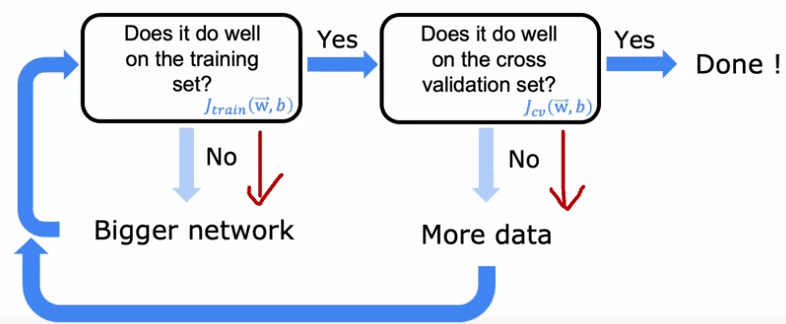
There are limitations to this recipe, such as the cost of training bigger neural networks and the availability of more data. However, the rise of neural networks has been assisted by the rise of fast computers, including GPUs, which have been useful for speeding up the training process. This recipe also explains the rise of deep learning in recent years, as it has been successful in applications where a lot of data is available.

The bias-variance tradeoff is a fundamental concept in machine learning and neural networks offer a new way of addressing this dilemma. By training large neural networks on moderate-sized datasets, we can reduce bias or variance as needed without having to trade off between the two. However, this recipe has its limitations and it's essential to keep in mind that during the development of a machine learning algorithm, the bias and variance can change, and it's important to keep monitoring them.