Make your convolutional Neural Networks better

Introduction

In our previous articles, we focused on developing convolutional neural networks (CNNs) that excel at recognizing images in binary classes, such as distinguishing between horses and humans or cats and dogs. Despite working remarkably well, we must remain cautious of falling into the overconfidence trap induced by overfitting. This risk becomes particularly prominent when training CNNs with limited datasets. In this article, we will delve into the concept of overfitting, provide an example using TensorFlow, and explore effective techniques to address this challenge, starting with the power of data augmentation.

Understanding Overfitting:

Overfitting refers to a situation where a model becomes exceptionally proficient at recognizing specific patterns from a restricted dataset but struggles when faced with unfamiliar instances. To illustrate this concept, let's consider a scenario involving shoes. Suppose the only shoes you have ever encountered in your life are hiking boots. With this limited exposure, you have developed a clear understanding of what shoes look like based on this singular example. Consequently, if someone were to show you hiking boots of different sizes, you would easily identify them as shoes. However, if presented with a high-heel shoe, despite it being a shoe, you might fail to recognize it as such. In this case, your understanding of what constitutes a shoe has become overfit to the specific characteristics of hiking boots, rendering you inflexible to variations. Overfitting is a common challenge in training classifiers, especially when working with limited data.

Augmentation: Maximizing Dataset Effectiveness: To mitigate the risks associated with overfitting, we can employ various tools and techniques to make our smaller datasets more effective. One such approach is data augmentation. When working with CNNs, we typically apply convolutions to images to identify specific features, like pointy ears for cats or the number of legs for humans. Convolutions excel at identifying distinct features that are clearly visible in the image. However, what if we could go beyond that? What if we could manipulate the cat image to resemble other images of cats with differently oriented ears? By training the network with augmented images, we can increase its adaptability and improve its ability to recognize variations of a particular feature.

Example with TensorFlow:

Let's consider a practical example using TensorFlow to highlight the power of data augmentation. Suppose we have a dataset of cat images, but none of them depict a reclining cat. Without data augmentation, our CNN might struggle to identify a reclining cat since it was never exposed to such examples during training. However, by introducing augmentation techniques like image rotation, we can transform the upright cat images in our dataset, making them resemble reclining cats. This augmentation enhances the network's ability to detect reclining cats, even if no explicit reclining cat images were available for training. By expanding the dataset artificially through augmentation, we effectively introduce more diverse examples, reducing the risk of overfitting and enhancing the network's generalization capabilities.

Image augmentation

Image augmentation plays a crucial role in enhancing the performance of convolutional neural networks (CNNs) by introducing variations and increasing the adaptability of the model to different features. In our previous discussions, we explored the image generator class, which already incorporated some level of augmentation through resizing. However, there are additional options available to further augment the dataset. Let's examine some of these options and their potential impact on the training process.

Rotation Range: The rotation range parameter allows us to randomly rotate images within a specified range (0-180 degrees). By introducing random rotations, we can expose the network to images from different angles. For instance, specifying a rotation range of 0-40 degrees means that the images will rotate by a random amount between 0 and 40 degrees.
Shifting: Shifting involves moving the image within its frame. Many images have the subject centered, which can lead to overfitting if the model is trained solely on such images. To address this, we can randomly shift the subject within the image by a specified proportion of the image size. For example, offsetting the subject by 20 percent vertically or horizontally introduces variability and reduces the risk of overfitting to centered subjects.
Shearing: Shearing is a powerful augmentation technique that can help the model generalize to different orientations. Consider an image of a person in a particular pose that is absent from the training set. However, if we have a similar image with a comparable pose, we can shear the latter image by skewing it along the x-axis to achieve a similar pose. The shear_range parameter allows us to shear the image by random amounts, up to a specified proportion of the image size. For example, a shear range of 20 percent means the image can be sheared by up to 20 percent.
Zoom: Zooming in or out on an image can be an effective augmentation technique to improve the model's ability to recognize generalized examples. By zooming, we can spot details that might be missed at a broader scale. The zoom parameter specifies the relative portion of the image to zoom in on. For example, using a value of 0.2 means that the images will be randomly zoomed by up to 20 percent of their original size.
Horizontal Flipping: Horizontal flipping is a useful tool for increasing the structural similarity between images. It can help the model generalize to different orientations or poses. For instance, if our training data lacks images of women with their left hand raised but includes images with their right arm raised, horizontally flipping the latter images makes them more structurally similar to the former. By enabling random horizontal flipping, the images will be flipped at random during training.
Fill Mode: The fill mode parameter determines how to fill in any pixels that might be lost during augmentation operations. Using the "nearest" fill mode, which utilizes neighboring pixels, helps maintain uniformity in the image. However, there are other options available, and it's advisable to refer to the caret's documentation for further details.

for example:

 from tensorflow.keras.preprocessing.image import ImageDataGenerator

# Define the augmentation options
datagen = ImageDataGenerator(
    rotation_range=40,
    width_shift_range=0.2,
    height_shift_range=0.2,
    shear_range=0.2,
    zoom_range=0.2,
    horizontal_flip=True,
    fill_mode='nearest'
)

# Load and augment the images
train_generator = datagen.flow_from_directory(
    'path_to_training_data_directory',
    target_size=(150, 150),
    batch_size=32,
    class_mode='binary'
)

# Create and train the model using augmented data
model = create_model()  # Replace with your own model creation function
model.compile(optimizer='adam', loss='binary_crossentropy', metrics=['accuracy'])
model.fit(train_generator, epochs=10)

The Impact of Image Augmentation:

To observe the impact of image augmentation, let's examine a scenario involving training a model to classify cats versus dogs. We will compare the performance of models trained with and without augmentation. By evaluating both cases, we can assess the effectiveness of augmentation in improving the model's ability to generalize and avoid overfitting.

Transfer learning

In the previous sections and articles, we discussed the challenges of overfitting and explored techniques such as image augmentation to mitigate its effects. However, these approaches have limitations, especially when working with small training datasets. In such cases, transfer learning offers a powerful solution by leveraging pre-existing models trained on larger and more diverse datasets. Let's delve into the concept of transfer learning and its benefits.

Concept

Transfer learning involves taking an existing model that has been trained on a vast amount of data and using the features it has learned for a different task or dataset. Instead of building a model from scratch, we can utilize the convolutional layers of a pre-trained model that have already learned rich and useful features. By doing so, we can save time and resources while benefitting from the knowledge encoded in the pre-trained model.

Visualizing a typical model, we see a series of convolutional layers followed by a dense layer leading to the output layer. When employing transfer learning, we can incorporate someone else's pre-trained model, which may be more sophisticated and trained on a much larger dataset. These models come with intact convolutional layers that have already learned powerful features. Rather than retraining these layers on our own dataset, we can lock them and use them to extract features from our own data. This way, we can leverage the convolutional layers of a model trained on a large dataset to identify important features in our own data.

The process involves using the pre-trained model's learned convolutions to extract features from our data, followed by retraining the dense layers of the model using our dataset. By following this approach, we can benefit from the knowledge and feature extraction capabilities of a model trained on a vast amount of data, while adapting the final layers to suit our specific task.

Typically, the convolutional layers are locked to preserve the learned features. However, there is flexibility in deciding which layers to retrain. While the higher-level convolutional layers are often left locked, some lower-level layers can be retrained if they are too specialized for the specific images in our dataset. Experimentation and trial and error can help determine the optimal combination of locked and retrained layers.

One example of a well-trained state-of-the-art model is Inception, which has been pre-trained on the large-scale ImageNet dataset. ImageNet consists of 1.4 million images across 1,000 different classes, making it a valuable source of pre-existing knowledge for various computer vision tasks.

By leveraging transfer learning and utilizing pre-trained models like Inception, we can leverage the convolutional layers' learned features and adapt them to solve our specific classification problem with a smaller dataset.

Transferred features

All of the layers have names, so you can look up the name of the last layer that you want to use. If you inspect the summary, you'll see that the bottom layers have convolved to 3 by 3. But I want to use something with a little more information. So I moved up the model description to find mixed7, which is the output of a lot of convolution that are 7 by 7. You don't have to use this layer and it's fun to experiment with others. But with this code, I'm going to grab that layer from inception and take it to output.

 # Define new model
last_output = inception.get_layer('mixed7').output
x = Flatten()(last_output)
x = Dense(hidden_units, activation='relu')(x)
output = Dense(1, activation='sigmoid')(x)
model = Model(inception.input, output)

So now we'll define our new model, taking the output from the inception model's mixed7 layer, which we had called last_output. This should look exactly like the dense models that you created way back at the start of this course. The code is a little different, but this is just a different way of using the layers API. You start by flattening the input, which just happens to be the output from inception. And then add a Dense hidden layer. And then your output layer which has just one neuron activated by a sigmoid to classify between two items. You can then create a model using the Model abstract class and passing in the input and the layers definition that you've just created.

And then you compile it as before with an optimizer and a loss function and the metrics that you want to collect.

I won't go into all the codes to download cats versus dogs again, it's in the workbook if you want to use it. But as before you're going to augment the images with the image generator. Then, as before, we can get our training data from the generator by flowing from the specified directory and going through all the augmentations. And now we can train as before with model.fit_generator. I'm going to run it for 100 epochs.

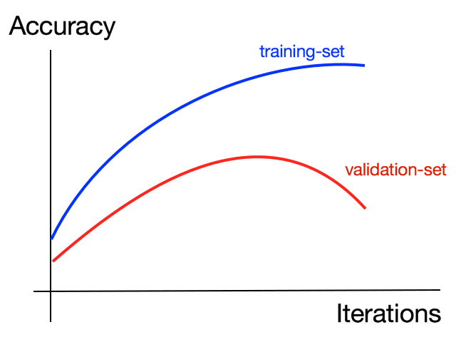
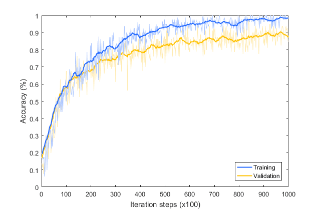
What's interesting if you do this, is that you end up with another but a different overfitting situation. Here is the graph of the accuracy of training versus validation. As you can see, while it started out well, the validation is diverging away from the training in a really bad way. So, how do we fix this? We'll take a look at that in the next lesson.

Dropouts

When we retrain the inception classifier features for cats versus dogs, we ended up over-fitting again. We also had augmentation, but despite that, we still suffered from over-fitting. So let's discuss some ways that we can avoid that in this lesson. Now here's the accuracy of our training set versus our validation set over 100 epochs. It's not very healthy.

There's another layer in Keras called a dropout. And the idea behind the dropout is that layers in a neural network can sometimes end up having similar weights and possibly impact each other, leading to over-fitting. With a big complex model like this, that's a risk. So if you can imagine the dense layers can look a little bit like this.

By dropping some out, we make it look like this.

And that has the effect of neighbors not affecting each other too much and potentially removing overfitting.

So how do we achieve this in code? Well, here's our model definition from earlier. And here's where we add the dropout. The parameter is between 0 and 1 and it's the fraction of units to drop.

Multiclass

In the last sections, we have been building a binary classifier. One which detects two different types of objects, horse or human, cat or dog, that type of thing. In this section, we'll take a look at how we can extend that for multiple classes.

Remember when we were classifying horses or humans, we had a file structure like this:

dataset

train

horses
humans

validation

horses
human

There were subdirectories for each class, where in this case we only had two.

The first thing that you'll need to do is replicate this for multiple classes like this:

dataset

train

rock
paper
scissors

validation

rock
paper
scissors

In these directories, we can put training and validation images for Rock, Paper, and Scissors.

How to

Once your directory is set up, you need to set up your image generator. Here's the code that you used earlier, but note that the class mode was set to "binary". For multiple classes, you'll have to change this to "categorical" like this:

 train_datagen = ImageDataGenerator(...)
train_generator = train_datagen.flow_from_directory(..., class_mode='categorical')

The next change comes in your model definition, where you'll need to change the output layer. For a binary classifier, it was more efficient to have one neuron and use a sigmoid function to activate it. Now, that doesn't fit for multi-class, so we need to change it. Now, we have an output layer that has three neurons, one for each of the classes (rock, paper, and scissors), and it's activated by softmax, which turns all the values into probabilities that will sum up to one. So the output of a neural network with three neurons and softmax activation would reflect the probabilities of each class.

 model.add(Dense(3, activation='softmax'))

The final change comes when you compile your network. Previously, your loss function was binary cross entropy. Now, you'll change it to categorical cross entropy like this:

 model.compile(loss='categorical_crossentropy', ...)

There are other categorical loss functions, including sparse categorical cross entropy, that you used in the fashion example, and you can also use those.

Train the model for 100 epochs, and you can observe the training progress with a chart. In this example, the training hits a maximum at about 25 epochs. So I'd recommend using a smaller number of epochs for efficiency.