Introduction

In today's digital age, the ability to understand and process human language has become a critical aspect of technological advancement. Natural Language Processing (NLP) stands at the forefront of this revolution, driving the development of intelligent systems that can comprehend and communicate with humans effortlessly. Through a combination of linguistics, computer science, and artificial intelligence, NLP enables machines to decipher the nuances of human speech and text, opening up a world of possibilities across various domains. From voice assistants that respond to our commands to chatbots that engage in meaningful conversations, NLP has emerged as a transformative force, reshaping the way we interact with technology. This article delves into the intricacies of NLP, highlighting its applications, challenges, and profound implications for industries and society as a whole. Join us as we unravel the power of NLP and explore how it is revolutionizing the future of human-machine communication.

Word based encodings

The Limitations of Character Encoding: Unlocking Word-level Meaning

When it comes to understanding the meaning of words using character encodings, the limitations quickly become apparent. Take, for example, the word 'LISTEN,' encoded using ASCII values.

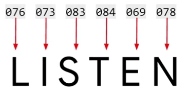
While this encoding captures the characters in the word, it fails to convey the semantics behind it. In fact, consider the word 'SILENT,' which shares the same letters as 'LISTEN' but has an entirely different meaning.

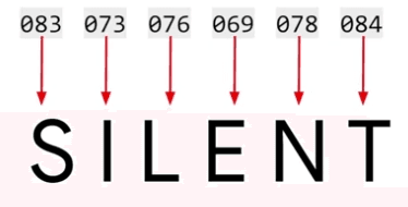
This demonstrates the inadequacy of character encodings in capturing word-level semantics.

Shifting to Word-level Encoding: A Promising Approach

To overcome the shortcomings of character encodings, a shift towards word-level encoding emerges as a more promising approach. By assigning a unique value to each word, we can capture the essence of the word and utilize these values for training a neural network. For instance, let's consider the sentence "I Love my dog." Assigning values to each word, such as 'I' as 1, 'Love' as 2, 'my' as 3, and 'dog' as 4, we can represent the sentence as the sequence 1, 2, 3, 4.

Flexibility in Sentence Encoding and Token Creation

Word-level encoding provides flexibility when encountering new sentences. Suppose we have the sentence "I love my cat." Since we have already encoded the words 'I love my' as 1, 2, 3, we can reuse these values. To represent 'cat,' which is a new token, we assign it the number 5. Comparing the encodings of the two sentences, 'I love my dog' is represented as 1, 2, 3, 4, while 'I love my cat' becomes 1, 2, 3, 5. This similarity between the sentence encodings forms a foundation for training neural networks based on words.

Simplifying the Process with TensorFlow and Keras APIs

Thankfully, frameworks like TensorFlow and Keras provide convenient APIs that simplify the process of word-level encoding and neural network training. These tools enable researchers and developers to leverage word values effectively and build robust models capable of understanding and processing human language at a deeper level.

By adopting word-level encoding, we can unlock a more nuanced understanding of language and lay the groundwork for more sophisticated natural language processing systems. In the following sections, we will delve deeper into the applications, techniques, and advancements in NLP that leverage word-level encoding, propelling us closer to bridging the gap between humans and machines.

Tensorflow

 import tensorflow as tf
from tensorflow import keras
from keras.preprocessing.text import Tokenizer

sentences = [
    'I love my dog',
    'I love my cat'
]

tokenizer = Tokenizer(num_words=100)
tokenizer.fit_on_texts(sentences)
word_index = tokenizer.word_index
print(word_index)

• Encoding Sentences: The tokenizer's fit_on_texts method is used to encode the provided sentences. It analyzes the text data and generates the necessary word encodings based on their frequency.

• Word Index Dictionary: After encoding the sentences, the tokenizer provides a word_index property, which returns a dictionary containing key-value pairs. Each key represents a word, and the corresponding value is its token.

• Handling Punctuation and Capitalization: The tokenizer automatically handles punctuation and capitalization. It treats words with different punctuation or capitalization as the same word, ensuring consistency in the encodings.

• New Text and Tokenization: If new text is introduced, the tokenizer seamlessly incorporates it into the existing word index. It assigns tokens to any new words and maintains the previous encodings.

Result :

 {'i': 1, 'love': 2, 'my': 3, 'dog': 4, 'cat': 5}

Text to sequence

To begin, let's create a list of sequences by encoding sentences using the generated tokens. For demonstration purposes, I've updated the code we've been working on. Notice that all previous sentences consisted of four words, but now we'll introduce a longer sentence. In the code snippet below, I simply invoke the tokenizer to convert the texts into sequences, resulting in the following output:

 import tensorflow as tf
from tensorflow import keras
from keras.preprocessing.text import Tokenizer

sentences = [
    'I love my dog',
    'I love my cat',
    'You love my dog!',
    'Do you think my dog is amazing ?'
]

tokenizer = Tokenizer(num_words=100)
tokenizer.fit_on_texts(sentences)
word_index = tokenizer.word_index

sequences = tokenizer.texts_to_sequences(sentences)

print(word_index)
print(sequences)

Result :

 {'my': 1, 'love': 2, 'dog': 3, 'i': 4, 'you': 5, 'cat': 6, 'do': 7, 'think': 8, 'is': 9, 'amazing': 10}
[[4, 2, 1, 3], [4, 2, 1, 6], [5, 2, 1, 3], [7, 5, 8, 1, 3, 9, 10]]

Upon running the code, you'll observe a new dictionary at the top, containing tokens for additional words like "amazing," "think," "is," and "do." At the bottom, the list of sentences has been encoded into integer lists, where tokens replace the original words. For example, "I love my dog" becomes "4, 2, 1, 3." An important aspect to note is that the text_to_sequences function can handle any set of sentences, encoding them based on the learned word set from the training data. This functionality becomes particularly valuable when performing inference with a trained model, as the input text must be encoded using the same word index for meaningful results.

Inference and Word Index Consistency:

Consider the following code snippet. Can you predict the outcome?

 # Try with words that the tokenizer wasn't fit to
test_data = [
    'i really love my dog',
    'my dog loves my manatee'
]

# Generate the sequences
test_seq = tokenizer.texts_to_sequences(test_data)

# Print the word index dictionary
print("\nWord Index = " , word_index)

# Print the sequences with OOV
print("\nTest Sequence = ", test_seq)

# Print the padded result
padded = pad_sequences(test_seq, maxlen=10)
print("\nPadded Test Sequence: ")
print(padded)

Upon running the code, the output would be as follows:

 [[4,2,1,3],[1,3,1]]

In the provided examples, the sentence "I really love my dog" remains encoded as "4, 2, 1, 3," while the word "really" is lost because it does not exist in the Word Index. On the other hand, "my dog loves my manatee" gets encoded as "1, 3, 1," representing "my dog my."

Dealing with Unseen Words and Padding

To avoid undesirable sentence structures like "my dog my," it's essential to have a diverse and extensive training dataset. A broad vocabulary is necessary to capture the nuances of language effectively. By exposing the neural network to a wide range of examples, we increase the chances of generating coherent sentences. The quality and size of the training data play a crucial role in achieving this objective.

Handling Unseen Words

In some cases, it's beneficial to handle unseen words instead of disregarding them entirely. Rather than ignoring these words, we can assign a special value to represent them. This can be accomplished by utilizing a property called "oov_token" in the tokenizer constructor. By specifying an "oov" (out-of-vocabulary) token, we indicate that any words not present in the word index should be represented by this token. It's important to select a unique and distinguishable value that won't be confused with an actual word. Let's take a look at an example:

 tokenizer = Tokenizer(num_words=100, oov_token="<OOV>")

By running this code, the resulting test sequences would resemble the following:

 {'<OOV>': 1, 'my': 2, 'love': 3, 'dog': 4, 'i': 5, 'you': 6, 'cat': 7, 'do': 8, 'think': 9, 'is': 10, 'amazing': 11}
[[5, 3, 2, 4], [5, 3, 2, 7], [6, 3, 2, 4], [8, 6, 9, 2, 4, 10, 11]]

For instance, the first sentence becomes "i out of vocab, love my dog," and the second sentence becomes "my dog oov, my oov." Although the syntax is not perfect yet, it demonstrates an improvement by incorporating the "oov" token. As the training corpus expands and more words are included in the word index, the coverage for previously unseen sentences is expected to improve.

Padding for Uniformity

Similar to the need for uniform image sizes when training with pictures, text data also requires a level of uniformity before training with neural networks. To achieve this, we can rely on the concept of padding. Padding involves adding special tokens or values to sentences to ensure they all have the same length. This process aligns the text data and makes it compatible with neural network architectures. By padding, we can treat sentences as uniform units during training, enabling effective learning and processing.

Padding

To begin, we need to import the pad_sequences function from tensorflow.keras.preprocessing.sequence. Once the tokenizer has generated the sequences, we can pass them to pad_sequences to apply padding. Here's an example of how to use it:

 from tensorflow.keras.preprocessing.sequence import pad_sequences

# Code snippet to generate sequences using the tokenizer

# Padding the sequences
padded_sequences = pad_sequences(sequences)

The result is a clear representation of the padded sequences. You can observe that the list of sentences has been transformed into a matrix, where each row has the same length.

 {'<OOV>': 1, 'my': 2, 'love': 3, 'dog': 4, 'i': 5, 'you': 6, 'cat': 7, 'do': 8, 'think': 9, 'is': 10, 'amazing': 11}
[[5, 3, 2, 4], [5, 3, 2, 7], [6, 3, 2, 4], [8, 6, 9, 2, 4, 10, 11]]
[[ 0  0  0  0  0  0  5  3  2  4]
 [ 0  0  0  0  0  0  5  3  2  7]
 [ 0  0  0  0  0  0  6  3  2  4]
 [ 0  0  0  8  6  9  2  4 10 11]]

The padding process inserts the appropriate number of zeros at the beginning of the sentence. For instance, a sentence like "5-3-2-4" requires no padding, while longer sentences may not need any padding either. It's worth noting that in some examples, the padding occurs after the sentence rather than before. If you prefer the latter approach, you can modify the code by adding the parameter padding='post'.

Setting Maximum Length and Handling Exceeding Sentences

By default, the width of the resulting matrix matches the length of the longest sentence. However, you can override this behavior using the maxlen parameter. For instance, if you want to limit your sentences to a maximum of five words, you can set maxlen=5. It's important to consider that if you have sentences longer than the specified maximum length, information will be lost. By default, the truncation occurs at the beginning of the sentence (truncating='pre'). If you prefer to truncate from the end, you can utilize the truncating='post' parameter.

Handling More Complex Data:

So far, we've demonstrated the encoding, padding, and handling of previously unseen sentences using hardcoded data examples. However, let's acknowledge that real-world scenarios often involve more complex data. In the next section, we will explore how to apply these techniques to handle more intricate and diverse datasets.

Sarcasm Detection

Public datasets are invaluable resources for training neural networks, offering real-world data and insights. In this article, we will explore the process of preparing a public dataset specifically focused on sarcasm detection. Our dataset of choice is a fascinating CC0 public domain dataset created by Rishabh Misra, which can be found on Kaggle. With its straightforward structure and simplicity, this dataset is an ideal starting point for training a neural network.

The dataset consists of three essential elements: the sarcasm label, the headline, and the corresponding article link. While parsing the HTML content of the articles and removing scripts and styles is beyond the scope of this article, we will solely focus on the headlines. To facilitate data loading into Python, a slight modification to the dataset format is recommended. Alternatively, you can download the pre-formatted dataset provided in the accompanying code for this article.

Once the dataset is correctly formatted, loading it into Python becomes a straightforward task. The json library proves to be quite useful in this regard, enabling us to load and parse the dataset in JSON format effortlessly. Here's a step-by-step breakdown of the process:

1. Import the json library to handle JSON data.
2. Open the dataset file using the open() function.
3. Load the dataset using json.load(file), where file is the opened dataset file.
4. Create separate lists to store the sentences, labels, and URLs extracted from the dataset.
5. Iterate through the dataset using a for loop.
6. For each item in the dataset, extract the headline, is_sarcastic label, and article link, and add them to the respective lists.

 with open("data/sarcasm.json", 'r') as f:
    datastore = json.load(f)

# Non-sarcastic headline
print(datastore[0])

# Sarcastic headline
print(datastore[20000])

sentences = []
labels = []
urls = []

for item in datastore:
    sentences.append(item['headline'])
    labels.append(item['is_sarcastic'])
    urls.append(item['article_link'])

By following these steps, you can efficiently structure the dataset, making it ready for further processing and training a neural network. The sentences can be used for tokenization, the labels for model training, and the URLs for additional analyses if needed.

Removing Stopwords

emoving stopwords is important when working with text data because these words typically do not carry significant meaning or contribute much to the context or classification of the text. Stopwords are commonly used words in a language, such as articles (e.g., "the", "a", "an"), conjunctions (e.g., "and", "but", "or"), prepositions (e.g., "in", "on", "at"), and other frequently occurring words.

By removing stopwords, we can reduce the dimensionality of the text data and focus on the words that are more informative and discriminative for the task at hand. This can lead to improved performance in natural language processing tasks such as text classification, sentiment analysis, topic modeling, and information retrieval.

Stopwords often appear in large quantities across different documents or texts, and their inclusion can introduce noise and make it harder for machine learning algorithms to identify patterns and extract meaningful features. Removing them allows the algorithm to focus on the more important words that carry the essence of the text.

Furthermore, removing stopwords can also help to improve computational efficiency. By eliminating common and less meaningful words, we can reduce the size of the data and speed up the processing time for various text analysis tasks.

However, it's worth mentioning that the set of stopwords can vary depending on the specific task, domain, or language being analyzed. Different languages have different sets of stopwords, and there may be domain-specific stopwords that need to be considered. Therefore, it's important to choose an appropriate stopwords list or even customize it based on the specific requirements of the task and the characteristics of the text data being processed.

     words = sentence.split()
    words = [word for word in words if word not in stopwords]
    sentence = ' '.join(words)

Embedding projector with classification

In this section we will explain how to construct a classifier of movie reviews. . The reviews can be categorized into two primary groups: positive and negative. With the assistance of labels, TensorFlow effectively generated embeddings that exhibit a distinct clustering of words specific to each review type. By conducting word searches, we can observe the illumination of certain clusters and identify associated words that clearly indicate a positive or negative classification. For instance, when searching for "boring," we can observe its prominence within a cluster alongside words like "unwatchable," which unmistakably belong to the negative category. Similarly, a search for a negative term like "annoying" would reveal its presence, along with related words, in the cluster specifically associated with negative reviews. Conversely, a search for "fun" would lead us to the discovery that "fun" and "funny" are positive, "fundamental" is neutral, while "unfunny" unequivocally falls into the negative category.

Dataset

A crucial aspect of TensorFlow's vision to facilitate the learning and usage of machine learning and deep learning is the inclusion of built-in datasets. There exists a library called TensorFlow Data Services (TFDS), which houses numerous datasets spanning various categories. For instance, there is a wide range of image-based datasets, as well as a selection of text datasets. In our upcoming tasks, we will utilize the IMDB reviews dataset, which proves to be an excellent choice.

Here is the dataset link : Large Movie Review Dataset

Let's load the dataset :

 import tensorflow_datasets as tfds

# Load the IMDB Reviews dataset
imdb, info = tfds.load("imdb_reviews", with_info=True, as_supervised=True)

The dataset is divided into 25,000 samples for training and 25,000 samples for testing. Each of these sets consists of iterables containing the respective sentences and labels stored as tensors. To utilize Keras tokenizers and padding tools, some conversion is necessary. Firstly, we define lists to hold the sentences and labels for both training and testing data. We can then iterate over the training data to extract the sentences and labels. Since the values are tensors, we can use the NumPy method to obtain their actual values. The same process is performed for the test set. Let's create our data:

 train_data, test_data = imdb['train'], imdb['test']
# Initialize sentences and labels lists
training_sentences = []
training_labels = []

testing_sentences = []
testing_labels = []

# Loop over all training examples and save the sentences and labels
for s,l in train_data:
  training_sentences.append(s.numpy().decode('utf8'))
  training_labels.append(l.numpy())

# Loop over all test examples and save the sentences and labels
for s,l in test_data:
  testing_sentences.append(s.numpy().decode('utf8'))
  testing_labels.append(l.numpy())

# Convert labels lists to numpy array
training_labels_final = np.array(training_labels)
testing_labels_final = np.array(testing_labels)

We proceed to tokenize the sentences. The hyperparameters are placed at the top for easy modification, making it more convenient than searching through function sequences to change literal values. The tokenizer and pad sequences are imported as before. An instance of the tokenizer is created, specifying the vocabulary size and the desired out-of-vocabulary token. The tokenizer is then fitted on the training set to build the word index.

 # Parameters
vocab_size = 10000
max_length = 120
embedding_dim = 16
trunc_type='post'
oov_tok = "<OOV>"

#  Initialize the Tokenizer class
tokenizer = Tokenizer(num_words = vocab_size, oov_token=oov_tok)

# Generate the word index dictionary for the training sentences
tokenizer.fit_on_texts(training_sentences)
word_index = tokenizer.word_index

Once the word index is obtained, the strings containing words in the sentences are replaced with their corresponding token values, resulting in a list called "sequences."

 # Generate and pad the training sequences
sequences = tokenizer.texts_to_sequences(training_sentences)
padded = pad_sequences(sequences,maxlen=max_length, truncating=trunc_type)

# Generate and pad the test sequences
testing_sequences = tokenizer.texts_to_sequences(testing_sentences)
testing_padded = pad_sequences(testing_sequences,maxlen=max_length, truncating=trunc_type)

As the sentences have varying lengths, the sequences are padded or truncated to ensure uniform length, determined by the maxlength parameter. The same process is applied to the testing sequences. It is important to note that the word index is derived from the training set, so the test data may contain more out-of-vocabulary tokens.

Now it is time to define the neural network, which should be familiar by now, except for the "embedding" line.

 # Build the model
model = tf.keras.Sequential([
    tf.keras.layers.Embedding(vocab_size, embedding_dim, input_length=max_length),
    tf.keras.layers.Flatten(),
    tf.keras.layers.Dense(6, activation='relu'),
    tf.keras.layers.Dense(1, activation='sigmoid')
])

# Setup the training parameters
model.compile(loss='binary_crossentropy',optimizer='adam',metrics=['accuracy'])

# Print the model summary
model.summary()

The embedding layer is a crucial component for text sentiment analysis in TensorFlow, where the transformation of words into dense vectors in a lower-dimensional space occurs, enabling the magic of sentiment analysis.

In text sentiment analysis, words with similar meanings tend to appear close to each other in a sentence. We can represent words as vectors in a higher-dimensional space, such as 16 dimensions, where words found together have similar vectors and cluster together. These word vectors are learned by the neural network during training and associated with sentiment labels, resulting in word embeddings.

To classify the sentiment of a sentence, we create a 2D array of word embeddings, with the sentence length and embedding dimension (e.g., 16). We can flatten this array or use global average pooling 1D to prepare it for classification. Global average pooling 1D calculates the average across the vector to flatten it.

Using global average pooling 1D makes the model summary simpler and potentially faster. With this approach, you can achieve a training accuracy of 0.9664 and a test accuracy of 0.8187 over 10 epochs, with each epoch taking about 6.2 seconds. Alternatively, using flatten can yield a training accuracy of 1.0, a validation accuracy of around 0.83, and each epoch taking about 6.5 seconds. Although slightly slower, the flatten approach tends to be more accurate.

Let's train and visualize our embedding :

 #training
num_epochs = 10
# Train the model
model.fit(padded, training_labels_final, epochs=num_epochs, validation_data=(testing_padded, testing_labels_final))

#Visualize
# Get the embedding layer from the model (i.e. first layer)
embedding_layer = model.layers[0]

# Get the weights of the embedding layer
embedding_weights = embedding_layer.get_weights()[0]

# Print the shape. Expected is (vocab_size, embedding_dim)
print("embedding_weights.shape")
print(embedding_weights.shape)

The result will be :

 embedding_weights.shape
(10000, 16)

Let's begin by extracting the results of the embeddings layer, which corresponds to layer zero in our model. We retrieve the weights of this layer and print their shape, which in this case is a 10,000 by 16 array. This indicates that our corpus contains 10,000 words, and we are working with a 16-dimensional embedding space.

To plot these embeddings, we need to reverse our word index. Currently, the word index has the word as the key and the corresponding token as the value. To decode the tokens back into words, we need to flip the word index:

 # Get the index-word dictionary
reverse_word_index = tokenizer.index_word

Next, we write the vectors and metadata auto files. These file types are recognized by the TensorFlow Projector, which enables us to visualize the embeddings in 3D space. In the vectors file, we write the coefficient values of each dimension for every word embedding. The metadata file contains the words themselves.

To view the results, visit the TensorFlow Embedding Projector website at projector.tensorflow.org Click on the "Load data" button located on the left side of the screen. In the file dialog, select the vector.TSV file for the vectors and the meta.TSV file for the metadata. Once the data is loaded, you will see a visualization similar to the one described.

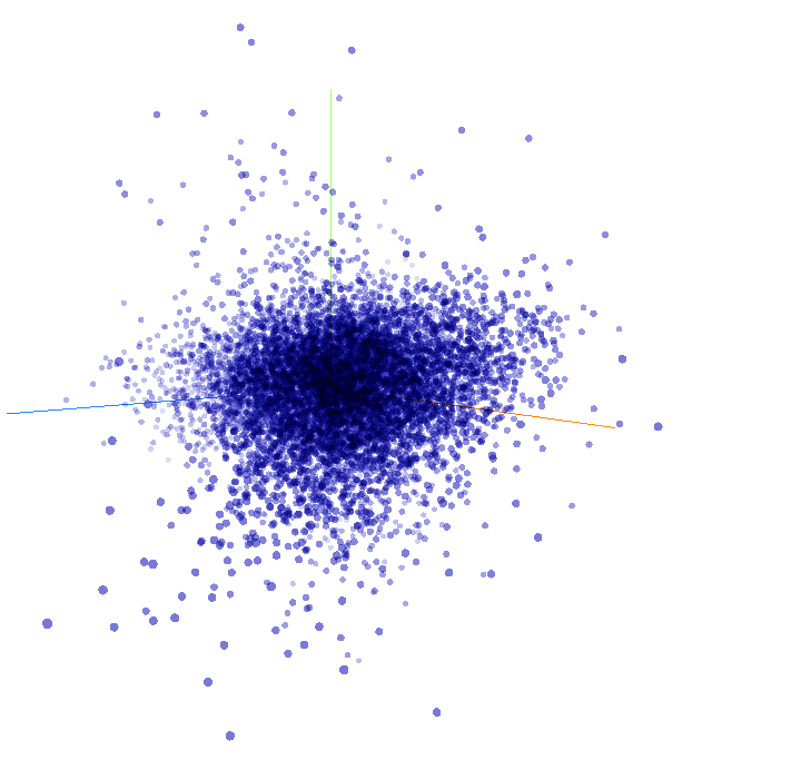
To enable the binary clustering of the data, tick the "sphereize data" checkbox on the top left. This option allows you to observe the clustering of words. Feel free to experiment by searching for specific words or clicking on the blue dots representing words in the chart. The goal is to explore and have fun with the visualization.

Subwords

Fortunately, some data scientists have already prepared the IMDb dataset for us. In this video, we'll explore a pre-tokenized version of the dataset, where the tokenization is done on subwords. This is interesting because it highlights the unique challenges of text classification, where the sequence of words can be just as crucial as their individual presence.

SubwordTextEncoder

SubwordTextEncoder is a type of tokenizer used in natural language processing tasks, particularly for text classification. It addresses the challenge of tokenizing words in a way that captures both the individual words and meaningful subword units.

Unlike traditional tokenizers that split text solely based on white spaces or punctuation, SubwordTextEncoder breaks words down into smaller subword units. This is particularly useful for handling out-of-vocabulary (OOV) words, rare words, or words that have morphological variations.

Add neuronal

We now have a pre-trained sub-words tokenizer available. To examine its vocabulary, we simply access its sub-words property. To understand how it encodes or decodes strings, we can utilize the encode and decode methods, respectively. This reveals the tokenization process by printing the encoded and decoded strings.

 # Encode the first plaintext sentence using the subword text encoder
tokenized_string = tokenizer_subwords.encode(training_sentences[0])
print(tokenized_string)

# Decode the sequence
original_string = tokenizer_subwords.decode(tokenized_string)

# Print the result
print (original_string)

If we wish to see individual tokens, we can decode each element separately, showcasing the value-to-token association. Keep in mind, this tokenizer respects case sensitivity and punctuation, which is a departure from the previous tokenizer we reviewed.

Now, let's shift our attention to applying this tokenizer for IMDB classification. The model structure we will use should look familiar by now. However, it's important to consider the shape of the vectors emerging from the tokenizer through the embedding layer, as they can't be easily flattened. Therefore, we will employ Global Average Pooling 1D.

 # Build the model
model = tf.keras.Sequential([
    tf.keras.layers.Embedding(tokenizer_subwords.vocab_size, embedding_dim),
    tf.keras.layers.GlobalAveragePooling1D(),
    tf.keras.layers.Dense(6, activation='relu'),
    tf.keras.layers.Dense(1, activation='sigmoid')
])

Following standard procedures, you can compile and train the model. The result visualization can be achieved with the provided code, and the graphs generated should resemble a particular pattern.

 import matplotlib.pyplot as plt

# Plot utility
def plot_graphs(history, string):
  plt.plot(history.history[string])
  plt.plot(history.history['val_'+string])
  plt.xlabel("Epochs")
  plt.ylabel(string)
  plt.legend([string, 'val_'+string])
  plt.show()

# Plot the accuracy and results
plot_graphs(history, "accuracy")
plot_graphs(history, "loss")

An interesting aspect of sub-word tokenization is that individual sub-words often lack sensible meaning. It's only when they're sequenced together that they produce semantically meaningful information. Consequently, a strategy that allows learning from sequences could significantly enhance our model's performance.

Sequence models

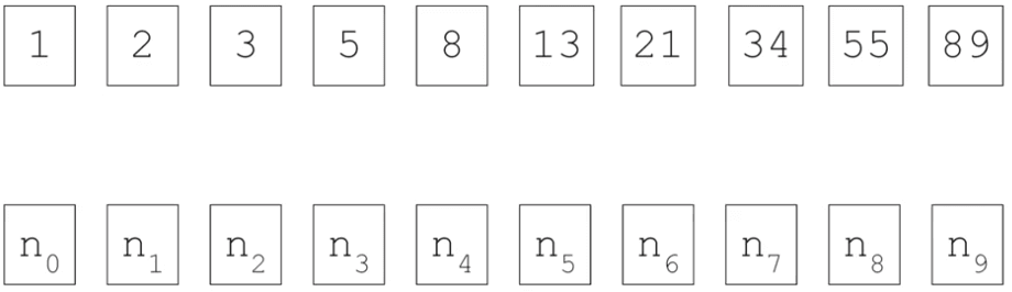
In the field of artificial intelligence, neural networks serve as powerful functions that learn rules from input data and corresponding labels. This allows us to leverage these learned rules for various tasks. However, traditional neural networks do not consider the importance of sequential information. To grasp the significance of sequences, let's explore the Fibonacci sequence—an ordered set of numbers. We can replace the specific values with variables like n_0, n_1, n_2, and so on, to denote them. In this sequence, each number is the sum of the two preceding numbers. For instance, 3 equals 2 plus 1, 5 equals 2 plus 3, 8 equals 3 plus 5, and so forth.

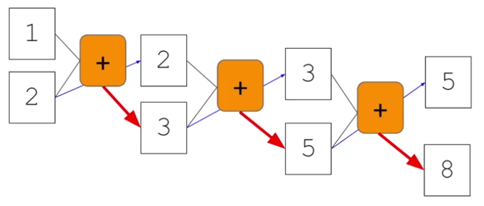
To represent this process visually, we can imagine that the numbers one and two are input into a function, resulting in the number three. The second number, two, is carried over to the next step, where it combines with three to yield five. This pattern continues, with each output becoming part of the next step's input. This concept shares similarities with recurrent neural networks (RNNs).

An RNN, depicted as x as input and y as output, incorporates a feedback loop where the output from a previous step becomes an input for the next step. This becomes clearer when we connect multiple RNNs in a chain-like structure. For example, x_0 is input into the function, producing output y_0. This output then serves as input, along with x_2, for the next function, resulting in output y_2.

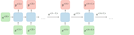
This process continues, allowing the network to maintain and process information from previous steps. Consequently, this forms the foundation of recurrent neural networks (RNNs).

LSTMs (Long Short-Term Memory)

An inherent limitation arises when employing conventional approaches for text classification. Consider the following scenario: "The sun is shining and the sky is a mesmerizing shade of azure." What word would likely come next? Most likely, "blue." The description of the sky as "a mesmerizing shade of azure" provides a crucial clue in this context.

However, let's examine another sentence: "During my travels in Japan, I immersed myself in their rich culture and learned how to eat something." How would you complete that sentence? While one might suggest "sushi," a more accurate response would be "ramen." The mention of Japan and the reference to immersing in their rich culture provide the necessary context for understanding the preferred cuisine.

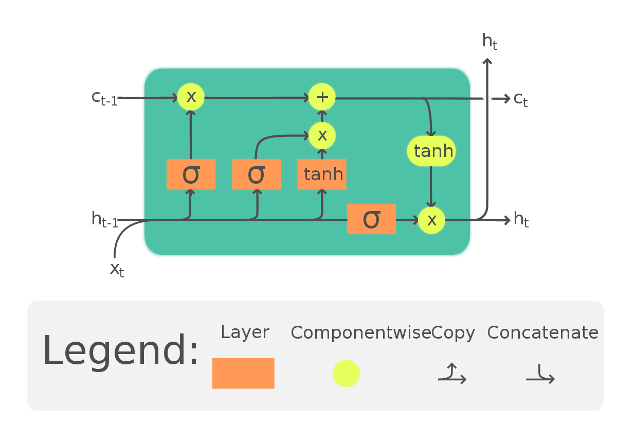
To address such challenges, an update to recurrent neural networks (RNNs) has been developed, known as long short-term memory (LSTM). LSTMs go beyond simply passing the context, as in RNNs, by introducing an additional pathway called the "cell state." This pathway enables the network to retain and utilize context from earlier tokens, mitigating issues where the relevant context appears further away in the sentence. Moreover, cell states can be bidirectional, allowing later contexts to influence earlier ones. We will explore code implementations to better understand the bidirectional impact on context.

Implementing LSTM

Now, let's delve into the implementation of LSTMs in code. Below is an example of a model where I've added a second layer as an LSTM using tf.keras.layers.LSTM. The parameter passed to the LSTM layer represents the desired number of outputs, which in this case is 64. By wrapping it with tf.keras.layers.Bidirectional, we enable the cell state to propagate in both forward and backward directions. You'll observe this bidirectional behavior when exploring the model summary, depicted as follows:

 model = tf.keras.Sequential()
model.add(tf.keras.layers.Embedding(input_dim=vocab_size, output_dim=embedding_dim, input_length=max_seq_length))
model.add(tf.keras.layers.Bidirectional(tf.keras.layers.LSTM(64)))
model.add(tf.keras.layers.Dense(64, activation='relu'))
model.add(tf.keras.layers.Dense(num_classes, activation='softmax'))

model.summary()

The model summary showcases an embedding layer followed by a bidirectional LSTM, then two dense layers. Notably, the output from the bidirectional LSTM is now 128, even though we initially specified 64 outputs for the LSTM layer. This doubling occurs due to the bidirectional nature, which combines outputs from both the forward and backward directions.

It's also possible to stack LSTMs similar to other Keras layers. To achieve this, you need to include the return_sequences=True parameter in the first LSTM layer. This ensures that the outputs of the LSTM match the expected inputs of the subsequent layer. Here's an example:

 model = tf.keras.Sequential()
model.add(tf.keras.layers.Embedding(input_dim=vocab_size, output_dim=embedding_dim, input_length=max_seq_length))
model.add(tf.keras.layers.LSTM(64, return_sequences=True))
model.add(tf.keras.layers.LSTM(32))
model.add(tf.keras.layers.Dense(num_classes, activation='softmax'))

model.summary()

By incorporating the return_sequences=True parameter in the first LSTM layer, you maintain the sequence information and provide suitable inputs for the following layer in the stack.

Single LSTM vs multiple LSTM

Now, let's compare the accuracies between a one-layer LSTM and a two-layer LSTM over 10 epochs.

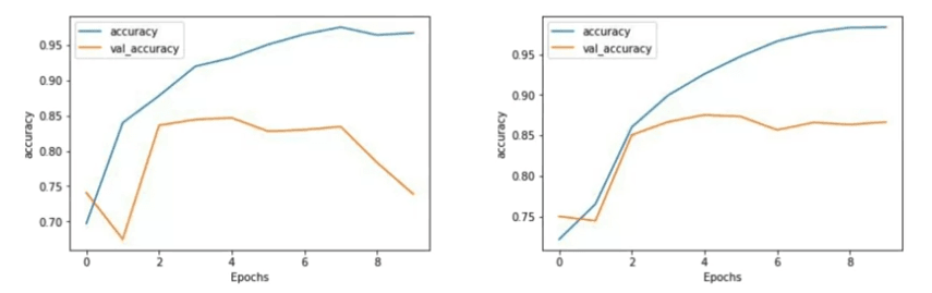
Although there isn't a significant difference in accuracy, we can observe a notable distinction in the validation accuracy curve. Notice that the training curve for the two-layer LSTM appears smoother. In my experience training networks, jaggedness in the curve can be indicative of model improvements needed, and the single-layer LSTM in this case exhibits some roughness.

If we extend the training to 50 epochs, we can further analyze the results.

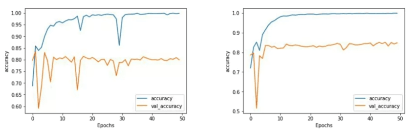
The one-layer LSTM demonstrates an increasing accuracy trend but is susceptible to sharp dips along the way. While the final accuracy might be good, these dips raise concerns about the overall accuracy of the model. On the other hand, the two-layer LSTM exhibits a much smoother accuracy curve, instilling greater confidence in its results.

It's worth noting the validation accuracy, which stabilizes at approximately 80 percent. Considering that both the training and test sets consist of 25,000 reviews, and we are using only 8,000 sub-words from the training set, there will be many tokens in the test set that are out of vocabulary. Yet, even with this challenge, we achieve an accuracy of around 80 percent.

The loss results show a similar pattern, with the two-layer LSTM exhibiting a smoother curve. The loss gradually increases with each epoch, indicating the need for careful monitoring to ensure it flattens out in later epochs, as desired.

 model = tf.keras.Sequential([
    tf.keras.layers.Embedding(vocab_size, embedding_dim, input_length=max_length),
    tf.keras.layers.GlobalAveragePooling1D(),
    tf.keras.layers.Dense(24, activation='relu'),
    tf.keras.layers.Dense(1, activation='sigmoid')
])

When I replaced the pooling layer with an LSTM, the results changed substantially. The model not only reached the previous benchmark of 85% accuracy swiftly but also continued improving, eventually reaching around 97.5% accuracy within just 50 epochs. While the validation set's accuracy did decrease somewhat over time, it remained comparable to the initial model without the LSTM. One interesting observation here was a slight overfitting, a common concern with LSTM that could be addressed with some fine-tuning.

Furthermore, the loss values of the models displayed different patterns. The non-LSTM model reached a healthy state quickly and then remained relatively stable. However, with the LSTM model, the training loss consistently decreased, but the validation loss increased over time. This could be another indication of overfitting in the LSTM network. Notably, while the accuracy of the prediction improved, the confidence in it slightly diminished.

When you experiment with different network types, it's crucial to adjust your training parameters accordingly. These aren't mere drop-in replacements; each change can significantly affect your model's performance and characteristics.

Convolutional network

Another type of layer that can be used is the convolutional layer, similar to how it is applied in image processing.

 model = tf.keras.Sequential()
model.add(tf.keras.layers.Embedding(input_dim=vocab_size, output_dim=embedding_dim, input_length=max_seq_length))
model.add(tf.keras.layers.Conv1D(filters=128, kernel_size=5, activation='relu'))
model.add(tf.keras.layers.GlobalMaxPooling1D())
model.add(tf.keras.layers.Dense(64, activation='relu'))
model.add(tf.keras.layers.Dense(num_classes, activation='softma

The code snippet provided demonstrates the usage of a convolutional layer in a network, which closely resembles the previous architecture. By specifying the desired number of convolutions, their size, and activation function, words are grouped based on the filter size (e.g., 5 in this case). Convolutions are learned to map word classifications to the desired output.

Training the network with convolutions yields even better accuracy than before, achieving close to 100 percent on the training set and around 80 percent on the validation set. However, as observed previously, the validation loss increases, indicating potential overfitting. Given the simplicity of the current network, this outcome is not surprising, and further experimentation with different combinations of convolutional layers is necessary to address this issue.

By revisiting the model and exploring the parameters, it becomes evident that we have 128 filters, each considering 5 words. Inspecting the model dimensions reveals that the input size was 120 words, and a 5-word filter shaves off 2 words from both ends, resulting in 116 remaining words. The specified 128 filters are visualized within the convolutional layer component of the model.