Introduction

In the vast realm of data analytics and machine learning, understanding sequences and time series data stands as a critical competency, paving the way for robust and accurate predictions. In the realm of finance, weather forecasting, economics, or even healthcare, our ability to comprehend the chronological order of events and discern patterns over time can significantly augment decision-making processes.

The intriguing world of sequences, time series, and prediction beckons, offering a blend of statistics, machine learning, and deep understanding of temporal patterns. This article will delve into these interconnected fields, examining how they function individually and symbiotically to enable sophisticated analysis and reliable forecasting in numerous disciplines.

We will explore the fascinating journey from simple sequences, uncovering the rich complexity within time series data, and arrive at the critical task of prediction, the act of foretelling the future based on the patterns of the past. Whether you're a seasoned data scientist, an aspiring analyst, or simply a curious reader, prepare for an enlightening exploration of these powerful analytical tools. Strap in for a journey across time, where data points serve as stepping stones into the future.

Time series

When we look at the world around us, we often see patterns that repeat over time — the changing seasons, the rise and fall of stock prices, the ebb and flow of tides, or even our daily routines. This rhythmic dance of repetition and progression is reflected in what we call a Time Series.

A time series is a collection of data points listed or indexed in a chronological sequence. The data is typically recorded at consistent, equally-spaced intervals. These intervals could be every minute, every hour, every day, every month, or even annually.

Now, a time series could be univariate or multivariate. When we record a single variable over time, we call it a Univariate Time Series. For instance, if we were to track the daily temperature over a year, we would end up with a univariate time series of temperatures.

However, when we monitor more than one variable over time, we end up with a Multivariate Time Series. An example of this would be if we recorded both the daily temperature and rainfall over a year. Here, temperature and rainfall are the variables, and together, they form a multivariate time series.

How it works with machine learning ?

So, what does machine learning have to do with time series? In reality, there's a vast realm of possibilities that we can explore using machine learning on time series data.

The most obvious application is predicting or forecasting future values based on existing data. Consider the birth and death rate chart for Japan. Predicting future values in this scenario can be incredibly helpful for government agencies. Such predictions aid in planning for a multitude of societal impacts, like retirement policies and immigration trends.

But the uses of time series analysis don't stop at forecasting future values. There are times when we might want to look backwards, to reconstruct past data points and understand the historical trajectory that has led us to our present state. This process is known as imputation.

Imputation can help us paint a more comprehensive picture of the past, even when some of the data may be missing. Let's look at our Moore's law chart:

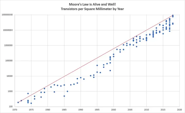
You might have noticed gaps in certain years where no data was available because no chips were released. Through imputation, we can fill these gaps and gain a more complete understanding of the data.

Beyond these applications, time series prediction can also serve as a valuable tool for anomaly detection. For example, imagine analyzing website logs; a sudden spike in a time series could indicate a potential denial-of-service attack.

Finally, time series analysis can also be used to identify patterns within the series, helping us understand the underlying mechanisms that generated the series. One classic application of this is in speech recognition, where we analyze sound waves (which are a type of time series) to identify words or sub-words. By training a neural network on this time series data, we can develop systems that accurately recognize and transcribe speech.

In essence, machine learning has a profound potential to transform our understanding and usage of time series data, from prediction and imputation to anomaly detection and pattern recognition.

Common patterns

Time series data come in a myriad of forms, each carrying unique patterns and narratives. It is beneficial to be able to identify these patterns as it helps us to understand the data and make accurate predictions. So, let's dive into some of the most common patterns we encounter in time series analysis.

trend

The first pattern we often see is a trend, where the time series moves in a specific direction. A classic example of this would be our earlier discussion on Moore's Law, which shows a consistent upward trend.

Seasonality

Another common pattern is seasonality, where a time series repeats itself at predictable intervals. A clear instance of this can be seen in the user activity data for a software development website, which exhibits regular dips — peaks during weekdays and troughs on weekends, illustrating a strong weekly cycle.

Some time series exhibit a blend of trend and seasonality. For example, a time series may have an overall upward trend but contain local highs and lows that correspond to seasonal changes.

White noise

But not all time series are predictable or contain discernible patterns. Some are a random assortment of values, a phenomenon referred to as 'white noise'. With this type of data, forecasting or prediction is next to impossible.

Autocorrelated

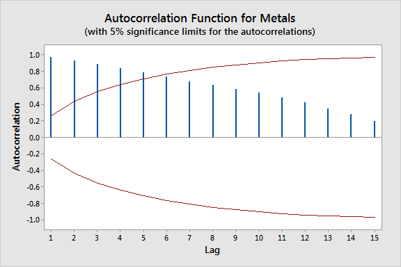
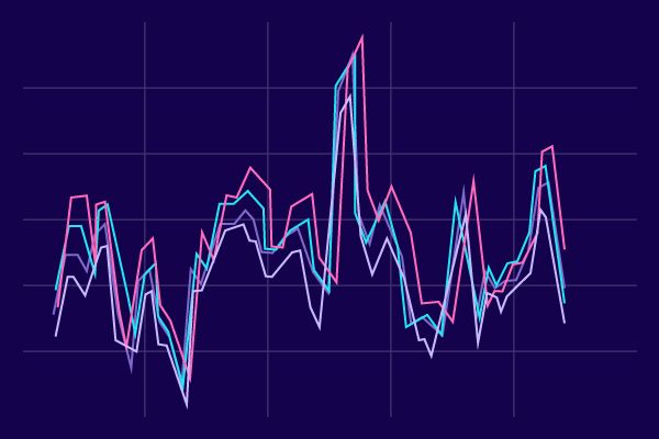
An intriguing type of time series is one that appears random with sudden spikes, but upon closer examination, shows an autocorrelated pattern. In such cases, the value at each time step is dependent on previous values. These series, which are said to have 'memory,' often contain unpredictable spikes or 'innovations'.

Real-life time series usually exhibit a mix of trend, seasonality, autocorrelation, and noise. By identifying these patterns, machine learning models can make meaningful predictions, assuming the future follows the same patterns as the past.

Mixing of patterns

However, time series can be complicated, changing behavior drastically over time. Such series, known as non-stationary time series, pose a unique challenge. For instance, a series might exhibit a positive trend and clear seasonality until a certain point, and then completely change its behavior, showing a downward trend without discernible seasonality.

In these scenarios, it's often more effective to train our models on a limited, recent period of the time series rather than the entire series. This is a deviation from the traditional machine learning approach where more data is considered better. In time series analysis, the value of data often depends on whether the series is stationary (its behavior doesn't change over time) or non-stationary.

Split data

Now that we've familiarized ourselves with the common patterns in time series, let's explore the methodologies we can employ to forecast them. We'll start with a realistic time series that incorporates trend, seasonality, and noise.

A simple way to forecast is to predict that the next value will be the same as the last one, a method known as naive forecasting. Despite its simplicity, this approach can provide a decent baseline. However, to evaluate our forecasting model, we need more sophisticated techniques.

One popular method is called fixed partitioning. We typically divide the time series into three segments: a training period, a validation period, and a test period. If the time series shows seasonality, we aim to ensure that each period contains a whole number of seasons (e.g., one, two, or three years if the series has yearly seasonality). This may seem different from how we usually partition data for non-time series datasets, but it effectively serves the same purpose.

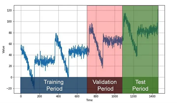
The model is trained on the training period and evaluated on the validation period. This is where we can experiment to find the right model architecture and tweak the hyperparameters until we achieve desirable performance. Once we've done that, we often retrain the model using both the training and validation data, then test it on the test period.

Interestingly, after testing, it's not uncommon to retrain the model using the test data too. Why? Because the test data, being the most recent, often provides the strongest signal for predicting future values. In fact, some may even forego the test set entirely and train the model using only the training and validation periods, with the future serving as the test set.

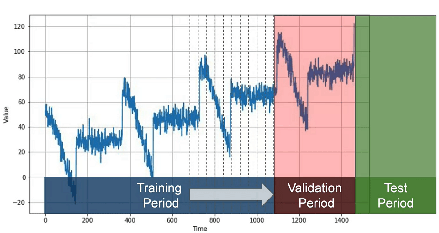
Another approach to partitioning is called roll-forward partitioning. This involves starting with a short training period and gradually increasing it at regular intervals, such as daily or weekly. At each iteration, the model is trained on the training period and used to forecast the next time unit in the validation period. This can be seen as doing fixed partitioning multiple times, continually refining the model in the process.

Evaluating performance

Once we've established our model and partitioned our data into distinct periods, the next step is to evaluate the model's performance. For this, we need a reliable metric.

A simple starting point is calculating the errors - the differences between the forecasted values from our model and the actual values over the evaluation period. However, we need a more standardized way of measuring these errors, and this is where several commonly used metrics come into play.

Mean Squared Error (MSE)

This metric involves squaring the errors and then calculating their mean. The purpose of squaring is to eliminate negative values, thus preventing errors from canceling each other out. For instance, if we have one error of +2 and another of -2, they would net out to zero, falsely implying no error. But if we square these errors, both would square to 4, correctly reflecting the presence of errors.

Root Mean Squared Error (RMSE)

Taking the square root of MSE returns the error calculation to the same scale as the original errors, giving us the RMSE.

Mean Absolute Error (MAE)

Another useful metric is the Mean Absolute Error or Mean Absolute Deviation. Instead of squaring the errors, MAE takes their absolute values`. This doesn't penalize large errors as much as MSE does. Depending on the specifics of your task, you might prefer the MAE or the MSE. For example:

• If large errors are potentially disastrous and much more costly than smaller ones, you might lean towards MSE.
• If your gains or losses are proportional to the size of the error, MAE might be a better choice.

Mean Absolute Percentage Error (MAPE)

The MAPE is the mean ratio between the absolute error and the absolute value. This metric provides an idea of the size of the errors relative to the values.

These metrics can be easily computed with code. For example, the Keras metrics library includes an MAE function. Given the synthetic data we presented earlier, we end up with an MAE of about 5.93.

Moving average and differencing

One common and straightforward forecasting method is calculating a moving average. The concept involves plotting the average of the values over a fixed period, known as an averaging window. This approach effectively reduces noise, providing a curve that roughly emulates the original series. However, it doesn't anticipate trend or seasonality, which can make it less accurate than naive forecasting under certain conditions.

To improve upon this, we can employ a technique known as differencing. Instead of examining the time series itself, we look at the difference between the value at time T and the value at an earlier period. This period could be a day, a month, a year, or any other relevant timeframe. When applied to our data, differencing removes trend and seasonality, yielding a new difference time series.

After obtaining this difference time series, we can use a moving average to forecast it. But remember, these forecasts are for the difference time series, not the original one. To retrieve the final forecasts for the original series, we add back the value at time T from the earlier period. This approach results in significantly improved forecasts.

Interestingly, our moving average forecasts are still quite noisy, even though they removed a lot of noise from the original series. This noise comes from the past values that we reintegrated into our forecasts. We can mitigate this by removing the past noise using a moving average on those past values as well.

When we implement this final step, we end up with much smoother forecasts and a significantly reduced mean absolute error. This surprisingly simple method gets us remarkably close to the performance of a perfect model.

This serves as a useful reminder: before diving headfirst into complex deep learning models, consider starting with simpler methods. Sometimes, they work just fine.

While we've examined moving averages using trailing windows so far, it's important to note that moving averages using centered windows can often be more accurate. A centered window takes into account the values before and after a particular point in time. However, using centered windows for smoothing present values isn't feasible, since we don't have access to future values.

Nonetheless, when it comes to smoothing past values, we can leverage the increased accuracy of centered windows. This is because we have access to the necessary future values when considering past points in time.

Having explored these statistical methods for predicting future values in a time series, it's essential to see these predictions in practice. That's where real-world implementation and hands-on practice come into play.

Forecasting

We're beginning our analysis with the Synthetic Dataset, where we'll employ statistical forecasting. Our goal is to generate a 'baseline', which we'll later aim to surpass with machine learning algorithms.

 import tensorflow as tf

# Assuming dataset is a DataFrame
dataset = tf.data.Dataset.from_tensor_slices(dataset.values)

Creating a Time Series with Trend, Seasonality, and Noise

Next, we aim to create a time series that includes trends, seasonality, and noise. These components represent common aspects found in many time series data.

 # Assuming trend, seasonal_pattern, and noise_level are defined functions
time = tf.range(len(dataset))
baseline = trend(time, slope=0.1) 
seasonality = seasonal_pattern(time)
noise = noise_level(time)

series = baseline + seasonality + noise

Here, we first establish a timeline with the same length as our dataset. We then generate a baseline trend, a seasonal pattern, and noise, and combine them into our time series.

Training Validation Set Split

To assess our models effectively, we split our data into a training set and a validation set. Here, we cut the data array at the 1,000th index.

 train_data = series[:1000]
valid_data = series[1000:]

This provides us with a training set of the first 1000 observations and a validation set of all subsequent data.

Naive Prediction

Our first forecasting approach, Naive Forecasting, presumes that the future value will be the same as the current one. We calculate the mean squared error (MSE) and the mean absolute error (MAE) as metrics to evaluate the performance of this naive forecast.

 naive_forecast = series[1:]

mse = tf.keras.metrics.mean_squared_error(series[:-1], naive_forecast).numpy()
mae = tf.keras.metrics.mean_absolute_error(series[:-1], naive_forecast).numpy()

print('Mean Squared Error:', mse)
print('Mean Absolute Error:', mae)

Here, we create a naive forecast by simply shifting the series one step into the future. We then calculate the MSE and MAE between the original series (excluding the last point) and the naive forecast.

Moving Average

We then explore another common forecasting approach, the Moving Average. It smooths out the series by calculating the average over a sliding window of data.

 def moving_average(series, window_size):
  forecast = []
  for time in range(len(series) - window_size):
    forecast.append(series[time:time + window_size].numpy().mean())
  return np.array(forecast)

moving_avg = moving_average(series, 30)

In this code, we define a function to calculate the moving average and apply it to our series. The window size of 30 implies we're averaging over the previous 30 points for each forecast.

Seasonality Adjustment and Improved Moving Average

Recognizing the seasonality of our data (with a span of one year or 365 days), we adjust our series by subtracting the series value 365 days prior from the current series value. We then reapply our moving average on this adjusted series and add back the past values to obtain a better prediction.

 diff_series = series[365:] - series[:-365]
diff_moving_avg = moving_average(diff_series, 50)

diff_moving_avg_plus_past = series[365:-50] + diff_moving_avg

mse = tf.keras.metrics.mean_squared_error(series[365:-50], diff_moving_avg_plus_past).numpy()
mae = tf.keras.metrics.mean_absolute_error(series[365:-50], diff_moving_avg_plus_past).numpy()

print('Mean Squared Error:', mse)
print('Mean Absolute Error:', mae)

Here, we first create the diff_series by subtracting the series value 365 days prior. Next, we calculate a moving average on this diff_series. By adding these moving averages back to the corresponding points in the past series, we get an improved forecast.

Deep learning with time series

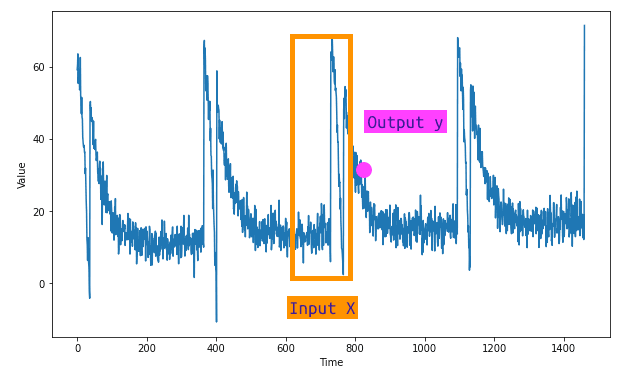
For any machine learning problem, the initial step is to split our data into features and labels. In time series forecasting, the feature refers to a certain number of sequential values in our dataset, while the label is the subsequent value in the series. This set of sequential values is also known as our window size—a snapshot of data that we use to train our machine learning model to predict the following value. As an illustration, if we're working with time series data over a 30-day period, we use the 30 values as the feature and the next value as the label. Subsequently, we train a neural network to correlate the 30 features with the single label.

We'll be using the tf.data.Dataset class to generate a dataset, which will initially comprise a range of 10 values. When visualized, this data series will run from 0 to 9.

 import tensorflow as tf

# Create a Dataset
dataset = tf.data.Dataset.range(10)

# Print each item in the dataset
for item in dataset:
    print(item.numpy())

result : 

0
1
2
3
4
5
6
7
8
9

To make the data more complex, we'll use the window method from the dataset class to enlarge our dataset. This method requires the window size and the shift amount as parameters. For instance, if we choose a window size of 5 and a shift of 1, the output will be a series of windows, such as 01234, 12345, and so on. When reaching the end of the dataset, windows with less than 5 values will appear due to a lack of data.

 import tensorflow as tf

# Create a Dataset
dataset = tf.data.Dataset.range(10)

# Apply the window method
dataset = dataset.window(5, shift=1)

# Print each window in the dataset
for window in dataset:
    for val in window:
        print(val.numpy(), end=" ")
    print()
    
result : 

0 1 2 3 4 
1 2 3 4 5 
2 3 4 5 6 
3 4 5 6 7 
4 5 6 7 8 
5 6 7 8 9 
6 7 8 9 
7 8 9 
8 9 
9 

To ensure a consistent window size, we can adjust the window method with an additional parameter—drop_remainder. By setting it to true, the method will omit all remainders, ensuring all windows contain five items. Our series will then start with 01234 and end with 56789. We can now convert these windows into numpy arrays to further prepare them for machine learning operations, which can be easily accomplished with the .numpy' method.

 import tensorflow as tf

# Create a Dataset
dataset = tf.data.Dataset.range(10)

# Apply the window method with drop_remainder
dataset = dataset.window(5, shift=1, drop_remainder=True)

# Batch the data and convert it to numpy arrays
dataset = dataset.flat_map(lambda window: window.batch(5))

# Print each window in the dataset
for window in dataset:
    print(window.numpy())
    
result : 

[0 1 2 3 4]
[1 2 3 4 5]
[2 3 4 5 6]
[3 4 5 6 7]
[4 5 6 7 8]
[5 6 7 8 9]

Next, we split the data into features and labels. It is logical for all values except the last in each window to be the feature, while the last value is the label. We can achieve this by using the mapping function. To further enhance our dataset, we can shuffle the data before training using the shuffle method.

 import tensorflow as tf

# Create a Dataset
dataset = tf.data.Dataset.range(10)

# Apply the window method with drop_remainder
dataset = dataset.window(5, shift=1, drop_remainder=True)

# Batch the data and convert it to numpy arrays
dataset = dataset.flat_map(lambda window: window.batch(5))

# Split the data into features and labels, and shuffle the data
dataset = dataset.map(lambda window: (window[:-1], window[-1:])).shuffle(buffer_size=10)

# Print each feature and label
for x, y in dataset:
    print("Feature: ", x.numpy(), "Label: ", y.numpy())
    
result

Feature:  [4 5 6 7] Label:  [8]
Feature:  [3 4 5 6] Label:  [7]
Feature:  [2 3 4 5] Label:  [6]
Feature:  [1 2 3 4] Label:  [5]
Feature:  [0 1 2 3] Label:  [4]
Feature:  [5 6 7 8] Label:  [9]

The final stage in data preparation involves batching the data with the batch method. For instance, choosing a batch size of 2 will divide the data into pairs, creating three batches in total. Each batch contains pairs of corresponding features and labels.

Windowed dataset into neural network

To handle a time-series data in TensorFlow, we can create a function named windowed_dataset. This function will take three arguments: series, window_size, and batch_size, as well as an additional shuffle_buffer parameter that will aid in data shuffling. Here's how we can define the function:

 import tensorflow as tf

def windowed_dataset(series, window_size, batch_size, shuffle_buffer):
    # Step 1: Create a dataset from the series
    dataset = tf.data.Dataset.from_tensor_slices(series)
    
    # Step 2: Use the window method
    dataset = dataset.window(window_size + 1, shift=1, drop_remainder=True)
    
    # Step 3: Flatten the data
    dataset = dataset.flat_map(lambda window: window.batch(window_size + 1))
    
    # Step 4: Shuffle the data
    dataset = dataset.shuffle(shuffle_buffer)
    
    # Step 5: Split into features and labels
    dataset = dataset.map(lambda window: (window[:-1], window[-1]))
    
    # Step 6: Batch the data
    dataset = dataset.batch(batch_size).prefetch(1)
    
    return dataset

Now let's unpack this function:

1. Create a dataset from the series: The first step involves creating a dataset from the time-series data using TensorFlow's tf.data.Dataset.from_tensor_slices method.

2. Window the data: Next, we apply the window method to the dataset to break it up into specific windows, each shifted by one timestamp. We ensure that all windows are the same size by setting drop_remainder to True.

3. Flatten the data: To make the data easier to work with, we flatten it into chunks using the flat_map method.

4. Shuffle the data: The data is then shuffled using the shuffle method. The shuffle_buffer parameter specifies the number of elements from the beginning of the sequence that should be loaded, from which a randomly selected element will be picked.

5. Split into features and labels: After shuffling, the dataset is split into features (all elements except the last one in each window) and labels (the last element in each window).

6. Batch the data: Finally, the data is batched into the specified batch_size, and the function returns this final prepared dataset.

This function will allow you to create a manageable representation of your time-series data, ready for training a machine learning model.

Single layer NN

Let's split our data into training and validation sets. Here we split it at the time step 1000.

 # Assume series is our time-series data
split_time = 1000
x_train = series[:split_time]
x_valid = series[split_time:]

Now we create and train a simple model:

 import tensorflow as tf
from tensorflow.keras.models import Sequential
from tensorflow.keras.layers import Dense
from tensorflow.keras.optimizers import SGD

# Set constants
window_size = 20
batch_size = 32
shuffle_buffer_size = 1000

# Create the windowed dataset
train_set = windowed_dataset(x_train, window_size, batch_size, shuffle_buffer_size)

# Define the model
l0 = Dense(1, input_shape=[window_size])  # A single dense layer
model = Sequential([l0])

# Compile the model
model.compile(loss="mse", optimizer=SGD(lr=1e-6, momentum=0.9))

# Train the model
model.fit(train_set, epochs=100, verbose=0)

# Print the weights
print("Layer weights: {}".format(l0.get_weights()))

The model has only one layer, l0, which is a dense layer with a single neuron. The layer is added to the model using the Sequential API. The model is compiled with mean squared error as the loss function and stochastic gradient descent as the optimizer. The learning rate and momentum for SGD are set to 1e-6 and 0.9, respectively.

Next, the model is trained on the train_set for 100 epochs. The verbose parameter is set to 0, so no training output is displayed.

Finally, the weights of the layer l0 are printed. The first array represents the weights (20 values in this case, corresponding to the window_size), and the second value is the bias. These values are learned by the network during training to best fit the data. The weights and bias values represent the parameters of the learned linear regression model.

Prediction

Let's delve into understanding the intricacies of using a single-layer neural network to calculate linear regression. Essentially, the weights and the bias in our model are used to make predictions based on the input data. For instance, given a series of 20 data points, our neural network model is trained to use these input values, apply the weights, add the bias, and generate a predicted output.

In the context of TensorFlow we can implement this easily. Here is a simple example:

 import tensorflow as tf
import numpy as np

# Assume x_values and y_values are your data points
x_values = np.random.rand(100)
y_values = x_values * 3 + 2 + np.random.randn(100)*0.1

# Define the model
model = tf.keras.models.Sequential([
    tf.keras.layers.Dense(1, input_shape=[1])
])

# Compile the model
model.compile(optimizer='sgd', loss='mean_squared_error')

# Fit the model
model.fit(x_values, y_values, epochs=10)

In this TensorFlow example, a single-layer neural network is created to perform linear regression. We train the model on our x and y values. The model learns to adjust its internal weights and bias to minimize the difference between the actual and predicted y values.

Post training, if we pass a series of 20 items from our data to this model, we can get a prediction:

 # Reshape your data
x_values_20 = x_values[:20].reshape(-1,1)

# Predict
predictions = model.predict(x_values_20)

Here, the reshaping of data with np.newaxis is necessary to match the input shape required by the model. model.predict then generates a predicted output for the given 20 values.

To make forecasts, we take the last window_size elements from the series, predict the next value, and append it to the series. We repeat this process to generate as many forecasts as required:

 forecasts = []
for time in range(len(series) - window_size):
    forecast = model.predict(series[time:time + window_size][np.newaxis])
    forecasts.append(forecast)

forecasts = forecasts[split_time-window_size:]
results = np.array(forecasts)[:, 0, 0]

We can create a plot to compare the actual vs predicted values:

 import matplotlib.pyplot as plt

plt.figure(figsize=(10,6))
plt.plot(x_values, y_values, 'b.')
plt.plot(x_values[:20], predictions, 'r-')
plt.show()

The blue dots represent the actual values and the red line represents our model's predictions.

We can also calculate the mean absolute error (MAE) to assess the quality of our predictions:

 mae = tf.keras.losses.mean_absolute_error(y_values[:20], predictions)
print('Mean Absolute Error:', mae.numpy())

Improve prediction

To continue from where we left off, we can leverage the power of a Deep Neural Network (DNN) to further improve our model accuracy. This example outlines the application of a simple three-layered DNN to perform a more accurate time-series forecast.

First, we need to generate our dataset. We use the previously defined windowed_dataset function and pass our training data (x_train), the desired window size, batch size, and shuffle buffer size.

 dataset = windowed_dataset(x_train, window_size, batch_size, shuffle_buffer_size)

The model is defined as a three-layered DNN with 10 neurons in each of the first two layers and 1 neuron in the final layer. The input shape is the size of the window and we're using ReLU (Rectified Linear Unit) as the activation function in each layer.

 model = tf.keras.models.Sequential([
    tf.keras.layers.Dense(10, activation="relu", input_shape=[window_size]),
    tf.keras.layers.Dense(10, activation="relu"),
    tf.keras.layers.Dense(1)
])

Then, we compile the model with a Mean Squared Error (MSE) loss function and Stochastic Gradient Descent (SGD) as the optimizer.

 model.compile(loss="mse", optimizer=tf.keras.optimizers.SGD())

We fit the model over 100 epochs and then calculate the Mean Absolute Error (MAE). If we find that the MAE has decreased, it indicates that we've made an improvement in our model's prediction capabilities.

One way we can further improve the learning efficiency and build a better model is by finding an optimal learning rate. For this, we introduce a learning rate scheduler as a callback function. This function adjusts the learning rate at the end of each epoch based on the epoch number.

 lr_schedule = tf.keras.callbacks.LearningRateScheduler(
    lambda epoch: 1e-8 * 10**(epoch / 20))
optimizer = tf.keras.optimizers.SGD(lr=1e-8, momentum=0.9)
model.compile(loss="mse", optimizer=optimizer)
history = model.fit(dataset, epochs=100, callbacks=[lr_schedule])

We can plot the loss per epoch against the learning rate per epoch to find the optimal learning rate, which is the one corresponding to the lowest and stable loss.

 lrs = 1e-8 * (10 ** (np.arange(100) / 20))
plt.semilogx(lrs, history.history["loss"])
plt.axis([1e-8, 1e-3, 0, 300])

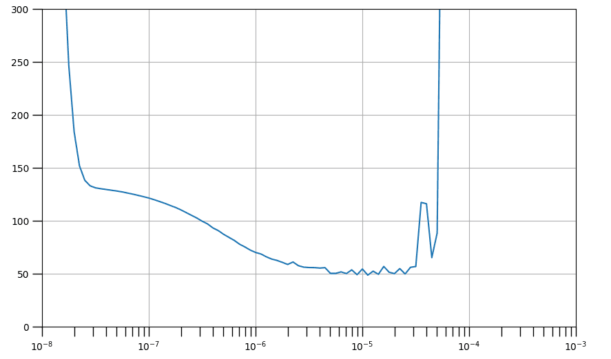
The graph presented above illustrates the assortment of learning rates that contribute to decreased losses, as indicated by a downward trend, and those that precipitate instability in the training process, which are depicted by jagged edges and an upward trajectory. Broadly, a point on a downward slope is optimal for selection as it suggests that the network continues to learn while maintaining stability. Selecting a point near the graph's minimum will expedite the training's convergence to that specific loss value, as will be demonstrated in the subsequent cells.

We will now proceed with the initialization of the same model architecture as before. You'll establish the optimizer with a learning rate approximating the minimum. It's initially set at 4e-6, but you're welcome to adjust this according to your findings.

 # Build the model
model_tune = tf.keras.models.Sequential([
  tf.keras.layers.Dense(10, activation="relu", input_shape=[window_size]),
  tf.keras.layers.Dense(10, activation="relu"),
  tf.keras.layers.Dense(1)
])

# Set the optimizer with the tuned learning rate
optimizer = tf.keras.optimizers.SGD(learning_rate=4e-6, momentum=0.9)

Next, compile and train the model as previously done. Pay close attention to the loss values and compare them with the output from your prior baseline model. It's highly probable that the final loss value of model_baseline will be achieved within the first 50 epochs of training this model_tune. After completing all 100 epochs, it's also likely that you'll observe a decreased loss.

 # Set the training parameters
model_tune.compile(loss="mse", optimizer=optimizer)

# Train the model
history = model_tune.fit(dataset, epochs=100)

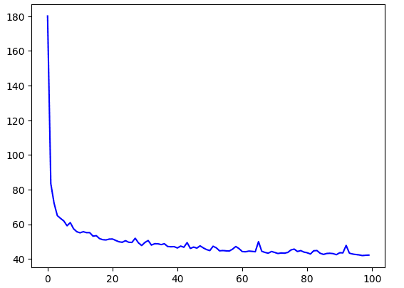
Let's plot it :

 # Plot the loss
loss = history.history['loss']
epochs = range(len(loss))
plt.plot(epochs, loss, 'b', label='Training Loss')
plt.show()

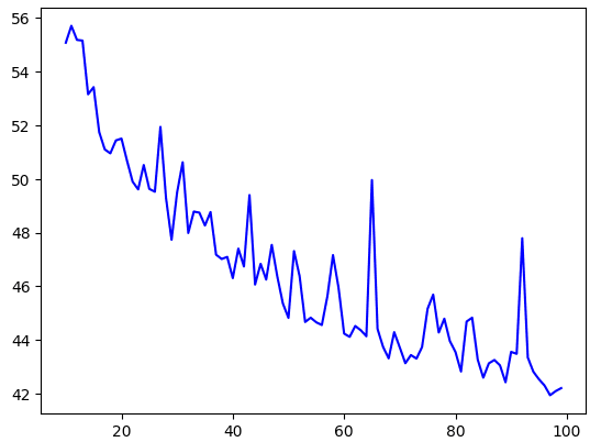
 # Plot all but the first 10
loss = history.history['loss']
epochs = range(10, len(loss))
plot_loss = loss[10:]
plt.plot(epochs, plot_loss, 'b', label='Training Loss')
plt.show()

You can get the preictions again and overlay it on the validation set.

 # Initialize a list
forecast = []

# Reduce the original series
forecast_series = series[split_time - window_size:]

# Use the model to predict data points per window size
for time in range(len(forecast_series) - window_size):
  forecast.append(model_tune.predict(forecast_series[time:time + window_size][np.newaxis]))

# Convert to a numpy array and drop single dimensional axes
results = np.array(forecast).squeeze()

# Plot the results
plot_series(time_valid, (x_valid, results))

Finally, calculate the metrics; you should obtain figures comparable to those from the baseline. If the results are significantly worse, the model might have overfitted. In that case, you can implement techniques to prevent this, such as introducing dropout.

 print(tf.keras.metrics.mean_squared_error(x_valid, results).numpy())
print(tf.keras.metrics.mean_absolute_error(x_valid, results).numpy())

Recurrent neural networks

Recurrent Neural Networks (RNNs) are a powerful type of neural network architecture designed to process sequential data. At the core of an RNN lies the recurrent layer, which enables the network to retain information about previous inputs as it processes new ones. This unique capability makes RNNs well-suited for handling sequences of data, such as time series. Unlike other neural networks, RNNs consider the temporal aspect of the data, taking into account the order and relationship between different time steps.

Architecture

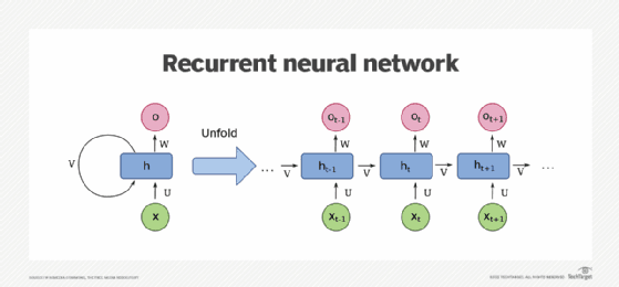
An RNN consists of one or more recurrent layers. Each layer contains a memory cell, which is responsible for storing information about past inputs. Although it may seem like there are multiple cells, in reality, there is just one cell that gets reused at each time step. This cell takes an input value for the current time step and produces an output along with a state vector. The state vector is then fed back into the cell at the next time step, creating a recurrent loop that allows information to flow through the network.

Applying RNNs to Time Series Analysis

In the context of time series analysis, an RNN can be used to forecast future values based on historical observations. By training the network on past data, it learns to capture the patterns and dependencies present in the time series. For univariate time series, where only one variable is considered, the input dimensionality is one. However, for multivariate time series, with multiple variables influencing the prediction, the input dimensionality increases accordingly.

The recurrent nature of RNNs is particularly beneficial in capturing temporal dependencies within a time series. Similar to how the position of a word in a sentence can affect its meaning in natural language processing, the proximity of values in a numeric series can also have a significant impact on predictions. RNNs excel at capturing these relationships, allowing them to make informed predictions based on the sequential nature of the data.

Three-Dimensional Inputs

When working with RNNs, the inputs are represented in a three-dimensional shape. To illustrate this, let's consider an example where we have a window size of 30 timestamps, and we are batching them in sizes of four. In this case, the shape of the input data would be 4x30x1. Each timestamp's input to the memory cell would be a 4x1 matrix, indicating a batch size of four and a single dimension for each time step.

The memory cell in an RNN takes both the current input and the previous output state matrix as its inputs. However, in the first time step, the previous state matrix would be initialized as zero. In subsequent steps, it would be the output from the memory cell at the previous time step.

The memory cell outputs both a Y value and a state vector. Suppose the memory cell comprises three neurons. In that case, the output matrix would be 4x3 because the batch size is four, and the number of neurons is three. Consequently, the full output of the layer would be three-dimensional, in this example, 4x30x3. Here, four represents the batch size, three represents the number of neurons, and 30 signifies the number of total steps.

The state output H is merely a copy of the output matrix Y. For instance, H_0 is a copy of Y_0, H_1 is a copy of Y_1, and so forth. At each timestamp, the memory cell receives both the current input and the previous output to perform computations.

In certain cases, you may only require a single vector output for each instance in the batch, despite inputting a sequence of data. This is commonly referred to as a sequence-to-vector RNN. In practice, achieving this is as simple as disregarding all outputs except the last one. When using frameworks like Keras in TensorFlow, this behavior is the default setting. If you want the recurrent layer to output a sequence instead, you need to explicitly specify return_sequences=True when creating the layer. This becomes necessary when stacking one RNN layer on top of another to propagate sequential information throughout the network.

Tensorflow

 # Build the Model
model_tune = tf.keras.models.Sequential([
  tf.keras.layers.SimpleRNN(20, return_sequences=True),
  tf.keras.layers.SimpleRNN(20, return_sequences=True),
  tf.keras.layers.Dense(1),
])

# Print the model summary
model_tune.summary()

Our exemplary RNN's first layer has return_sequences=True, allowing it to churn out a sequence. This output then serves as the feeding ground for the succeeding layer. However, the following layer doesn't have return_sequence set to True, hence it delivers an output at the final step only.

Paying attention to the input_shape parameter, we observe it is set to None and 1. In the TensorFlow world, the first dimension represents the batch size. The intriguing part here is that TensorFlow isn't fussy about the size, and you can skip defining it. The subsequent dimension symbolizes the number of timestamps. Setting this to None empowers the RNN to juggle sequences of diverse lengths. The final dimension is a singleton, reflecting the univariate nature of our time series.

Now, if we choose to set return_sequences to True across all the recurrent layers, an interesting shift happens. They all start outputting sequences, and consequently, the dense layer receives a sequence as its input. This behavior is managed by Keras by employing the same dense layer independently at each timestamp. This might give an illusion of multiple layers, but it's the very same one, reused at every time step. This intriguing arrangement gives birth to a sequence-to-sequence RNN, which ingests a batch of sequences and reciprocates with a batch of sequences, maintaining the same length.

 # Build the Model
model_tune = tf.keras.models.Sequential([
  tf.keras.layers.SimpleRNN(20, return_sequences=True),
  tf.keras.layers.SimpleRNN(20),
  tf.keras.layers.Dense(1),
])

# Print the model summary
model_tune.summary()

However, the dimensions might not always match perfectly. This depends on the number of units residing in the memory cell.

Lambda type

RNNs indeed are versatile, but sometimes we may need to add a touch of customization to better suit our tasks. This is where Lambda layers come in handy, giving us the freedom to perform arbitrary operations within the model definition itself, thereby enriching the capabilities of TensorFlow's Keras.

Firstly, let's address the mismatch in dimensions. Our window dataset helper function returns two-dimensional batches of windows - one for the batch size and the other for the number of timestamps. However, an RNN craves three dimensions - batch size, the number of timestamps, and the series dimensionality. This is where we can use a Lambda layer to add an extra dimension without having to modify our window dataset helper function. By setting the input shape to none, we're expressing that the model can consume sequences of any length.

Secondly, we'll deal with the scale of our outputs to aid training. RNN layers, by default, use the hyperbolic tangent (tanh) activation function, which restricts output values between -1 and 1. As our time series values usually hover in the tens (e.g., 40s, 50s, 60s, and 70s), rescaling our outputs to align with this range can boost learning. A Lambda layer provides the perfect canvas to accomplish this; we simply multiply the output by 100.

 import tensorflow as tf
from tensorflow.keras import layers

model = tf.keras.models.Sequential([
    layers.Lambda(lambda x: tf.expand_dims(x, axis=-1), input_shape=[None]),
    layers.SimpleRNN(20, return_sequences=True),
    layers.SimpleRNN(20),
    layers.Dense(1),
    layers.Lambda(lambda x: x * 100.0)
])

model.compile(optimizer='adam', loss='mse')

# Now your model is ready to be trained with your data

Adjusting learning rates

RNNs can be quite effective for time series predictions. For improving our model's training efficiency and prediction performance, we'll also be tweaking the learning rate of our neural network optimizer. This strategic approach can save substantial time in our hyper-parameter tuning.

We'll be training an RNN with two layers, each harboring 40 cells. To fine-tune the learning rate, we'll employ a callback that adjusts the learning rate slightly at the end of each epoch. In addition, we'll be using a new loss function, the Huber loss. This function is particularly useful when dealing with noisy data as it is less sensitive to outliers.

 # Define learning rate schedule
def lr_schedule(epoch):
    return 10 ** (epoch / 20)

lr_callback = LearningRateScheduler(lr_schedule)

model = tf.keras.models.Sequential([
    layers.Lambda(lambda x: tf.expand_dims(x, axis=-1), input_shape=[None]),
    layers.SimpleRNN(40, return_sequences=True),
    layers.SimpleRNN(40),
    layers.Dense(1),
    layers.Lambda(lambda x: x * 100.0)
])

optimizer = SGD(lr=1e-8, momentum=0.9)
model.compile(loss=tf.keras.losses.Huber(), optimizer=optimizer, metrics=["mae"])

history = model.fit(dataset, epochs=100, callbacks=[lr_callback])

Post 100 training epochs, we can ascertain our optimal learning rate for the Stochastic Gradient Descent (SGD) as somewhere between 10^-5 and 10^-6. We'll now train our model for 500 epochs using this learning rate and the SGD optimizer.

After the training, the chart showcasing the Mean Absolute Error (MAE) on the validation set presents an MAE of about 6.35. Though not bad, we should aim to do better.

Looking closer, we see that the trend of decreasing loss continues till around 400 epochs, after which it starts fluctuating. Given this, training for about 400 epochs should be enough.

Here's how we retrain our model with these settings:

 optimizer = SGD(lr=1e-5, momentum=0.9)
model.compile(loss=tf.keras.losses.Huber(), optimizer=optimizer, metrics=["mae"])
history = model.fit(dataset, epochs=400)

We notice that the MAE is slightly higher, but the time savings from 100 fewer epochs of training make it a fair trade-off. Evaluating the training MAE and loss shows promising results. Thus, even a simple RNN model can offer commendable performance.

LSTM

While our results with the simple RNN model were decent, there were peculiar plateaus in the predictions that indicate room for improvement. Despite experimenting with various hyperparameters, the improvement was modest. Now, let's shift gears and explore the potential of Long Short-Term Memory (LSTM) networks as an alternative to RNNs.

Recall our discussion on RNNs: they consist of cells that process batch inputs (X) and generate an output (Y) as well as a state vector. This state vector, along with the next input, gets passed on to the following cell, where it contributes to the computation of the next output and state vector. The state vector's influence, however, can wane over timestamps, which could be a potential drawback, especially for long sequences.

LSTMs tackle this diminishing influence by introducing a 'cell state' that perpetuates throughout the training process. This state is carried forward from cell to cell and timestamp to timestamp, ensuring better retention of the 'memory' of past data. As a result, data from earlier parts of the sequence can have a more substantial impact on the overall prediction compared to the case of simple RNNs.

Interestingly, LSTMs can also leverage bidirectional states, where the information flows both forwards and backwards. This approach has proven incredibly beneficial for text analysis. As for numeric sequence prediction, the advantage of bidirectional states isn't as clear-cut, making it an intriguing area for experimentation.

Transitioning from RNNs to LSTMs requires a few tweaks to our existing code. Let's unpack the changes:

 import tensorflow as tf
from tensorflow.keras import layers

tf.keras.backend.clear_session()

model = tf.keras.models.Sequential([
    layers.Lambda(lambda x: tf.expand_dims(x, axis=-1), input_shape=[None]),
    layers.Bidirectional(layers.LSTM(32, return_sequences=False)),
    layers.Dense(1),
    layers.Lambda(lambda x: x * 100.0)
])

optimizer = tf.keras.optimizers.SGD(lr=1e-6, momentum=0.9)
model.compile(loss=tf.keras.losses.Huber(), optimizer=optimizer, metrics=["mae"])

Initially, tf.keras.backend.clear_session() is used to clear any internal variables, ensuring our iterations don't interfere with each other. Following our dimension-expanding Lambda layer, we introduce a bidirectional LSTM layer with 32 cells. The output neuron then generates our prediction value. The learning rate is set to 1e-6, which is subject to further experimentation.

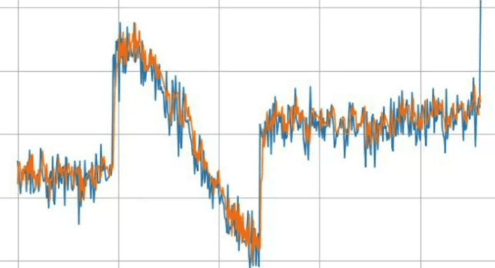
After running this LSTM model on our synthetic data, the results still exhibit a plateau under the major spike, and the MAE is moderately low. The predictions might also be somewhat underestimated.

To improve, we add another LSTM layer to our model:

 model = tf.keras.models.Sequential([
    layers.Lambda(lambda x: tf.expand_dims(x, axis=-1), input_shape=[None]),
    layers.Bidirectional(layers.LSTM(32, return_sequences=True)),
    layers.Bidirectional(layers.LSTM(32, return_sequences=False)),
    layers.Dense(1),
    layers.Lambda(lambda x: x * 100.0)
])

We must set return_sequences=True in the first LSTM layer for the second LSTM layer to work properly. The results now show a much better tracking of the original data, although it may slightly lag behind sharp increases. The MAE has also improved significantly.

Next, we add a third LSTM layer:

 model = tf.keras.models.Sequential([
    layers.Lambda(lambda x: tf.expand_dims(x, axis=-1), input_shape=[None]),
    layers.Bidirectional(layers.LSTM(32, return_sequences=True)),
    layers.Bidirectional(layers.LSTM(32, return_sequences=True)),
    layers.Bidirectional(layers.LSTM(32, return_sequences=False)),
    layers.Dense(1),
    layers.Lambda(lambda x: x * 100.0)
])

After training and running this updated model, we can compare the outputs and evaluate the benefits of having three LSTM layers.