Neurons

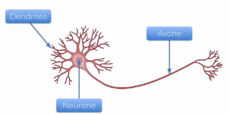
How can we recreate our neurons with a machine? First, we need to understand what a neuron is?

(https://res.cloudinary.com/dw6srr9v6/image/upload/v1636901352/neuroness_2f7ce27255.png)

• Dendrites: they serve a neuron to receive information
• Axons: they serve to send information to other neurons

You guessed it, neurons need to be several to function properly. Thus, the Dendrites and Axons allow the human brain to interact. But then how can it be represented?

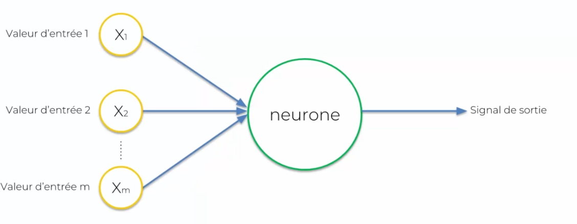
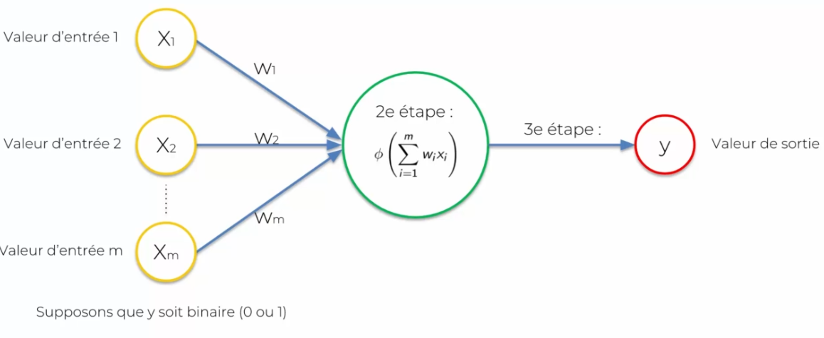
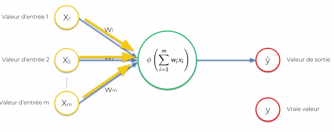
We no longer talk about dendrites or axons, but input values and output signals.

We no longer talk about dendrites or axons, but input values and output signals.

• Inputs will be represented in yellow
• The neuron will be represented in green

Each input will be represented by a neuron or data that will be given as input. The neuron will process this data to produce decisions: the output value (or signal). It is important to standardize our input values: we remove the mean divided by the standard deviation or by putting the variables on a variable from 0 to 1, we will come back later on this standardization. We also need to talk about the connection between the input values and the neuron: the weight. This weight must be continuously adjusted so that each input data, so that the neuron during these calculations can take into account the output data.

The activation function

The activation function is in the neuron to create an output value of the neuron. There are several:

Threshold function

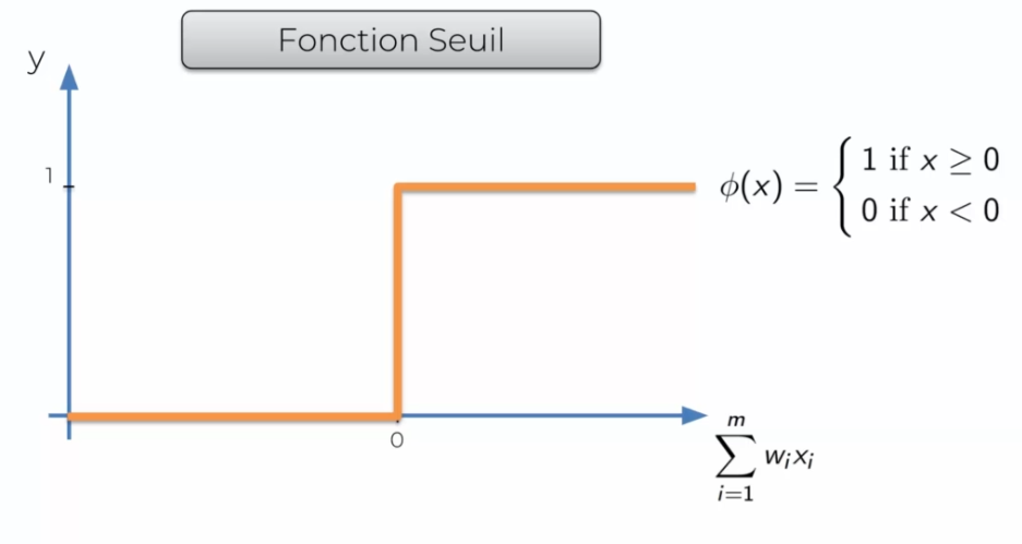
It is very simple, basically it will return 0 if the input signal is negative and 1 if it is possible or null.

Sigmoid function

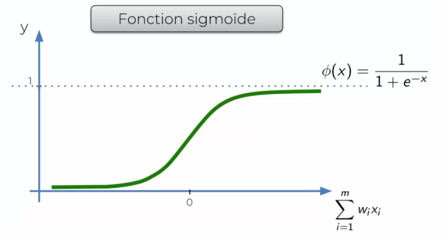
It is very similar to the Threshold function, but is smoother. It gradually reaches 1 and not directly. It is often used in the last layer, as it outputs a probability.

Rectifier function

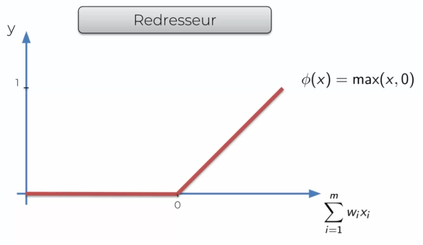
It is one of the most popular functions, if X is less than 0 it will cut the signal otherwise it will just return the signal.

Hyperbolic tangent (tanh)

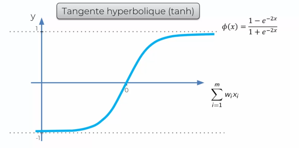
It is often used when we do not have a probability to output.

The most appropriate activation function?

In the following case:

We assume that the response is binary (0 or 1):

• Threshold activation function: it will return either 0 or 1
• Sigmoid activation function: it outputs a sort of probability and we can then decide on a rule

Let's move on to a more complicated case: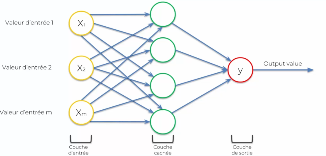

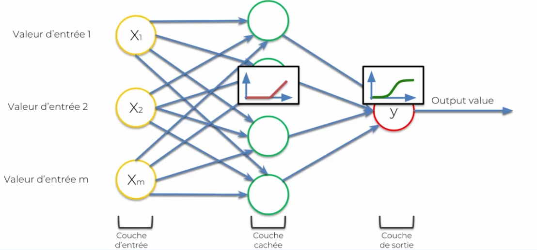
We see that we have more neurons, generally we will use:

• The rectifier function: it will allow depending on X, if it is high it will let it pass, otherwise it will block. Then on Y we will apply:
• The sigmoid function: which will allow applying a probability

The operation of a network

Let's imagine that we want to sell a house, we first ask ourselves:

• What will be the sale price of this house?

We assume that our neural network is trained (the weights on the synapses are defined). We will have several input variables:

• Surface (m2)
• Number of bedrooms (X2)
• Distance from the center (km)
• Age

We need to add hidden layers: all synapses are connected to a neuron, and sometimes they will have a weight different from 0. But how is it possible that some weights are 0? Because we will differentiate the inputs and assign each neuron a specialization. So for a neuron X, only certain synapses are relevant, while others are not. This is where the hidden layer comes in, which allows to specialize the input data based on a specific field, and reject (value 0) those that it no longer needs.

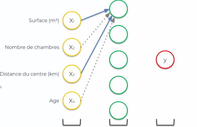
Combinations become important for a specific field, as it will allow a specific neuron to be specialized in field X and therefore output more precise data. Thus, the neural network will make decisions based on the input data.

Thus our hidden layer will pass the data directly to Y (output layer) which will result in a sale price.

The training of a network

If we take the previous neural network:

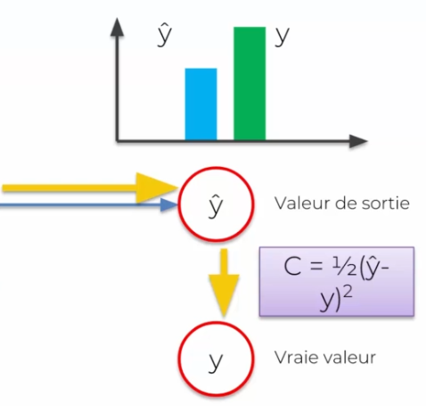
We notice that we changed y in output by ^y, this is because this value will be perceived as a prediction, while Y will be the real value.

• Real value means that it is an expected value during training
• Prediction means that it is the result obtained by our neural network

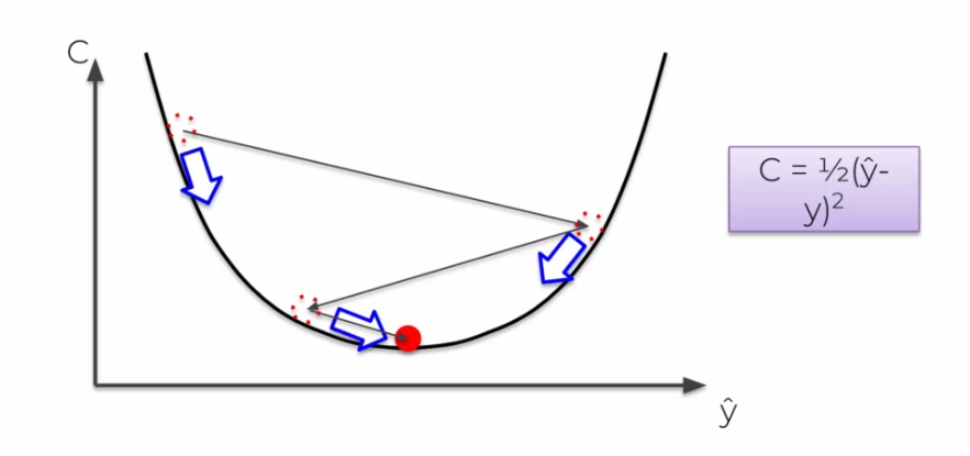
To then know if our value is good or not, we will compare it with the real value. We then apply a cost function:

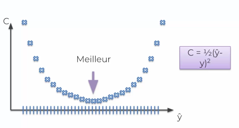
Our goal is to minimize the cost function as much as possible. To do this, after each cost, it is important to update the weight functions of each synapse. Why on the synapses? Because they are the only ones that can be updated. Each activation function will not have a direct impact.

This adjustment will allow us to know the cost of each synapse, adjust it and therefore reduce the final cost function to reduce the gap in ^Y and Y. Once the network is close to the true value, the training is considered complete and the network is ready to start.

Note: it is rare for the cost to be equal to 0!

But how does this work with multiple lines?

Training a neural network on multiple lines, multiple data, is called an epoch. How it works:

• Pass each line in the same neural network
• As the lines pass, we get multiple ^Y for each line
• We then calculate the cost value for all ^Y.
• We then sum up all the costs for each individual
• We propagate this information in the neural network and update the weight per individual

This entire process from left to right and updating the weights is called backpropagation.

The gradient algorithm

Previously we talked about cost functions, in our example we used a simple cost function. The brute force technique says that for a weight the best value is defined:

OK it works very well for one weight, but when we have several weights, we are affected by the curse of dimensionality. But how to minimize a cost function? That is, for many weight functions?

Suppose we try 1000 values per weight, which results in a lot of final combinations. It is currently impossible to calculate it, with a brute force system, by the best computer in the world.

To do this, we need the gradient algorithm. We make positive and negative tests (some iterations) to optimize the neural network, instead of testing everything one by one. We make iterations until we find the best value. Thus we solve a lot of calculation problems and in only a few iterations we reach the optimal solution.

The stochastic gradient algorithm

There is a problem with the gradient algorithm, we need a so-called convex curve for it to work. In the opposite case, we will have a local minimum in some cases that will not be a global minimum.

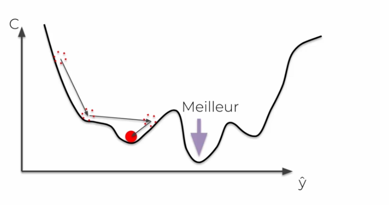
In the stochastic case, we add the cost directly line by line, so instead of making a final sum of the costs, at each iteration the weights are updated. It then avoids falling into global minima, it avoids fluctuations. It will also be + faster, and less deterministic than batch gradient.

Summarizing training

• Step 1: Initialize weights with values close to 0 (but not 0)
• Step 2: Send the first observation to the input layer, with a variable per
• Step 3: Forward Propagation (from left to right): Neurons are activated based on the weight assigned to them. Propagate the activations until the prediction ^Y is obtained.
• Step 4: The prediction is compared with the true value and the error is measured using a cost function.
• Step 5: Backpropagation (from right to left): The error is propagated back into the network and the weights are updated based on their responsibility in the error.
• Step 6: Repeat steps 1 to 5
• Step 7: When all the data has been passed through the ANN, it creates an epoch. Do more epochs to improve the neural network.

Regression and Classification

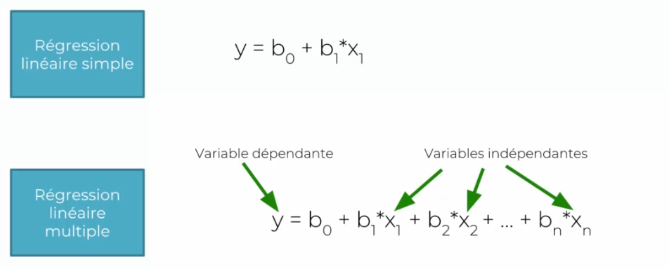
Simple Regression

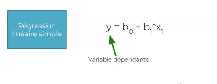
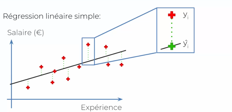
Take as an example: Y (dependent variable) is an employee's salary, what is the data (independent variable or X1) that makes this Y vary. Thus:

• Y: is the salary
• X1: is the employee's age, which increases their salary
• B1: is the coefficient of X1, showing how X affects Y
• B0: is a constant

We collect several data based on the years of the individuals. Take the following examples:

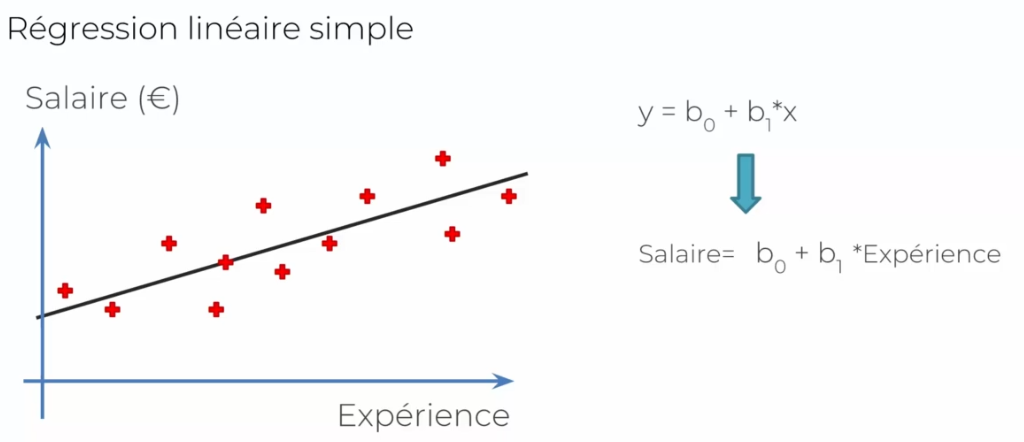
So we have a line in the graph that characterizes our norm that we are looking for. In this case, we simply draw a line as close to the middle as possible. Let's look at it from the ^Y (prediction) and true value side:

In this case, drawing a line is likely to be complex. We will never get a so-called relevant answer by drawing a line in the middle.

Multiple Regression

The method is the same, only the formula changes:

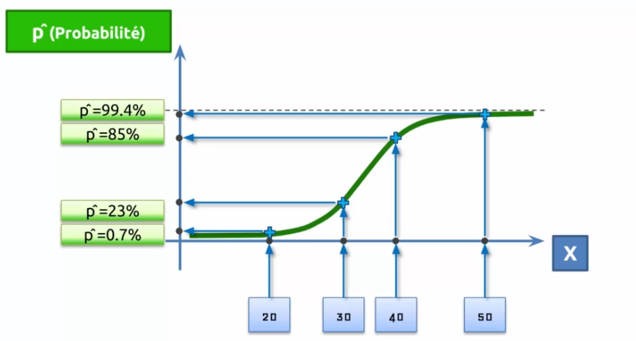
Logistic Regression

Suppose a company sends emails to customers and through this email, the customer buys or does not buy the offered offer:

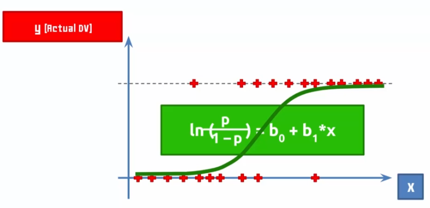
So we draw a curve that tries to minimize the errors, this curve is our model! If we talk about probability on the Y axis, we will say that the closer the curve is to Y, the more likely it is that our prediction is true.

Training a Neural Network

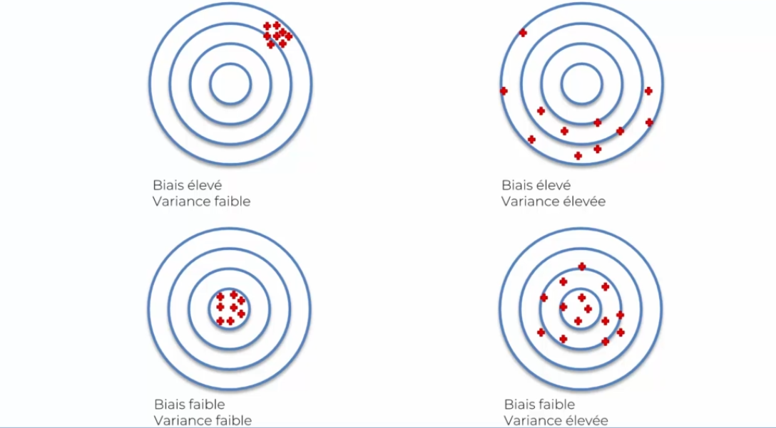
When evaluating a neural network multiple times, one notices that the success rate varies. This is due to the balance between bias and variance:

When evaluating a model, a good way to do so is by looking at the results through tests and emitted results. However, this is not the best approach as there will be a significant variance issue. So, another solution must be found: K-fold cross validation!

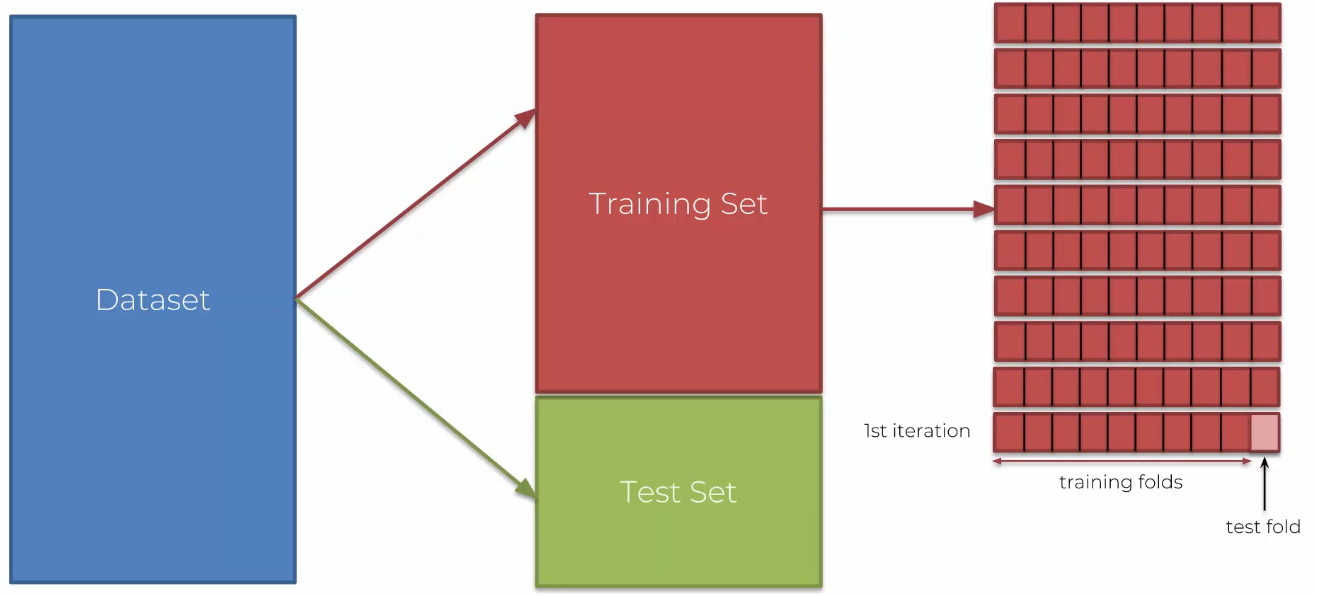
• We will take our dataset and not divide it into training and test data

• We will divide these data into 10 parts that will represent our dataset!

• At each iteration, we will take 9 parts for training and 1 for testing

• This way at each iteration the data changes and we have constantly different datasets

• So, we will have 10 values for accuracy, but also: more precise values, an idea of the value standard deviation (close to the mean). We will then know if we are close to variance, the goal being to have a low variance and low bias (accuracy).

It is important to understand that a neural network can be over-trained. One way to resolve this issue is to use: classifier.add(Dropout(0.1)), which allows for adding a chance variable where a neuron can be removed to add more complexity and prevent a neuron from getting too accustomed to results.

Adjusting a Neural Network

When evaluating a neural network several times, one notices that the success rate varies. This comes from the balance between bias and variance:

A good way to evaluate a model is to evaluate it by looking at the results through tests and outputs. But this is not the best, as we will have this issue of important variance. So we will have to find another solution: K-fold cross validation!

• We will take our data set that we will not divide into training and test data
• We will divide these data into 10 parts that will represent our data set!
• At each iteration, we will take 9 parts for our training and 1 for our test
• Thus at each iteration the data changes and we have constantly different data sets

• We will therefore have 10 values for accuracy, but also: more precise values, an idea of the value's standard deviation (very close to the average). We will then know if we are close to variance, the goal being to have a low variance and a low bias (accuracy).

One thing that is important to understand is that a neural network can be over-trained. One way to solve this issue is to use: classifier.add(Dropout(0.1)) which allows adding a chance variable where a neuron can be removed in order to add more complexity and thus avoid a neuron getting too used to results.

Adjusting a neural network

When creating a network, often one thinks that the first network created is the right one. But a network can always be improved by changing and testing parameters. Like:

• Adding or removing neurons
• Testing other activation functions To do this, a solution exists: Grid search. This algorithm allows testing several possibilities of parameters, and then outputting the best comparison.