Supervised vs Unsupervised

Machine Learning algorithms

During this article, we will learn about machine learning algorithms such as :

Supervised learning : It is the type of algorithm that is the most used used in real-world applications. They are more rapid advancements
Unsupervised learning
Recommender systems
Reinforcement learning

We will go through the different topics, and try to apply them into a context with many explications.

Supervised learning

Today 99% of value created by machine learning, is created by using supervised learning.

Regression

Let's explain it :

Consider to avoid an Input, called X, and an output called Y. We will explain to the machine, that we expect to have a Y variable, and to make it, we will create an algorithm which will help the machine to understand the need and how to solve it.

So Y here, is a prediction that the machine imagine to be the correct value. Let's take an example :

Input(X)	Output(Y)	Application
Email	spam?(0/1)	Spam filtering
Audio	text transcripts	Speech recognition
English	Spanish	Machine translation
Image, radar info	Position of the other car	Self driving car

We have here some example of this input / output applications. The main idea is to obtain a result that we already know and learn it to the machine.

After they learning about the example that you provide, for variable input and result output, we consider the training to be done. By the way, the AI should now able to receive new inputs and determined the correct answers (Y) by itself.

Imagine that you want to predict the housing price based on the house's size ?

We will collect some data existing
We will plot the data :

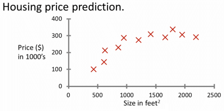
With this data, we have correct inputs and outputs, meaning that we have our dataset to provide to the AI.

So imagine this application, where we want to predict the price that we will sell a house. Lets take an example :

The easier way will be to draw a straight line between the different values, meaning that we have an average of the price. But it is not want we want, cause it can happens that you will sell you house for less or even for more and never sell it.
The most complicate way, will be to create a curve line, and includes the higher values to have an idea of the max that you can sell it. Which will reduce the risk, but can reduce the rapidity to sell too.

This is two approachs show you, the decision that you have to take, to drill with the perfect dataset that you think will be better for the learning.

During the supervised learning, we will provide an algorithm called : the right answer, which is the correct price Y given for every house on the plot. The role of this algorithm will be to predict, what is the best price to sell your house. This type of supervised learning is called Regression: we try to prediction a number infinitely many possible numbers.

Classification

Imagine that you have data regression to predict the Breast cancer detection :

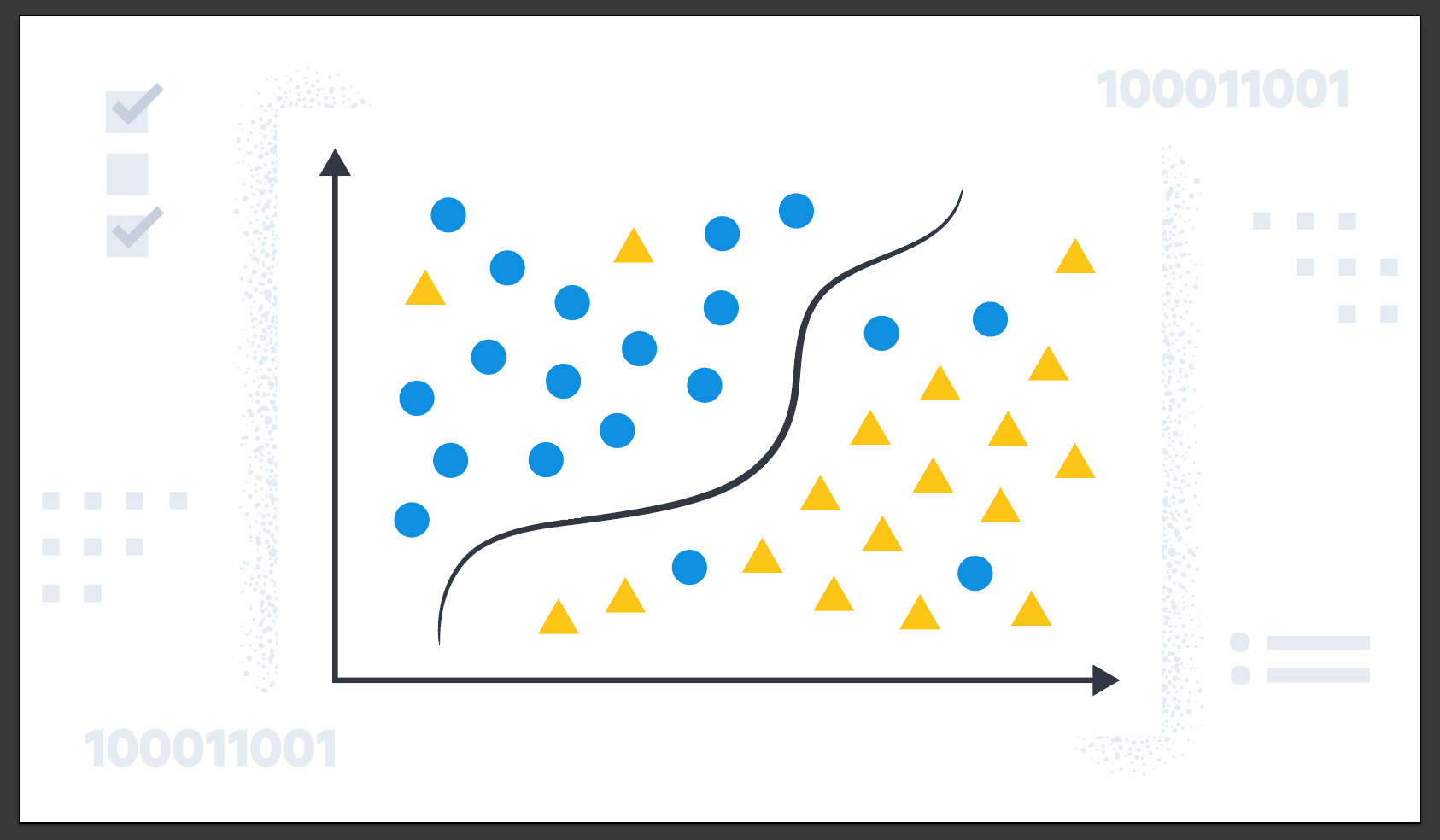
This AI, will be important for a doctor to detect a cancer earlier and save someone which need it. It will help to detect if a tumor that a lump is malignant meaning cancerous or dangerous.

So you should have data which enter data with different sizes :

Size	Diagnosis
2	0
5	1
1	0
7	1

0 means that it is bening
1 means that it is malignant

By using this data, we can create a plot, and you will see that the different between regression, will be that we try to predict small numbers: 2 possible outputs in this case. It is different from regression, where we try to predict infinitely numbers, here we have 2 possible solutions.

On the plot below, you see that we are using symbols, to denote the data, it is easier for us to have this kind of representativity.

During classification, you can have more than 2 outputs categories, maybe we can oputput multiple of cancer like :

Benign
Malignant type 1
Malignant type 2

In this case we can say that classification predicts categories which do not have numbers. Like, this pictures is a cat or a dog ? It can by the way predict a small limited set of possible output categories such as 0,1 and 2 but noit all possible numbers in between like 0.5 or 1.7.

Unsupervised learning

Unsupervised is I think just as super as supervised learning. When we do supervised learning, each input was link to an expected output value. In this unsupervised learning, we are not giving data, which are associated to output. So data only comes with inputs x, but not output labels y. The algorithm has to find structe in the data.

Clustering

We will to try to find interesting in unlabeled data. We asked the our room to figure out all by yourself what"s interesting or waht patterns or structures that might be in this data. Unsupervised will decide the data can be assigned to two different groups or two different clusters. And so it might decide, that there's one cluster what group over here, and there's another cluster or group over here. We call this type of unsupervised learning : clustering algorithm.

This algorithm is used by google news: every day, it goes and looks for hundred news on the internet, and groups related together. The clustering algorithm is finding articles, over internet, finding title article which mention a word and just group this informations together to provide a result.

Lets take a look to a clustering of DNA data, we have person with specific dna information, like the gene for eyes color,... By putting this data into algorithm to cluster some informations, which closed together, to create by itself a structure for each DNA data. It means that we do not provide any output, the model itself is creating the groups by analysing the data provided by X.

Anomaly detection

It is used to find unusual data points, this turns out to be really important for fraud detection, where unsual events, unsual transaction could be signs of fraud

##Dimensionality reduction

Compress data using fewer numbers, and avoid to lose as little information as possible.

Jupyter notebooks

It is the default environments that a lot of us use to code up and experiment and try things out. It provide the exactly same environment that huge companies are using over the world.

Linear regression model

You have introduce this model previously, we will go deeper inside the model and try to provide example that we will need.

It's probably the most widely used learning algorithm in the world today. Let's start with a problem that you can address using linear regression. Say you want to predict the price of a house based on the size of the house.

We receive this dataset from an agency, which is selling houses. Here each data point, each of these little crosses is a house with the size and the price that it most recently was sold for. Now, let's say you're a real estate agent and you're helping a client to sell her house. She is asking you, how much do you think I can get for this house? This dataset might help you estimate the price she could get for it.

You knows that the house id 1250 square feet, we can createa linear regression model from this dataset. Your model will fit a straight line to the data, which might look like this. Based on this, you trace that to the vertical axis on the left, you can see the price is maybe around here, say about 220,000$. This is an example, and linear is just an example to predict a range of possible numbers.

There is an example of data :

Size in feet²	Price in 1000$
2104	400
1416	232
1534	315
...
3210	870

Here you have inputs and outputs, from real data to define our data to ingest and the plots for predictions. It will be used to train the model and it is called: : the training set. So it is the support for model, or a set of inputs, called X : all values on "Size in feet²" is a X value. Where the price in 1000$ is the Y output variable.

To design a row, we will call a variable M, where M(i)= (X(i), y(i)) to design a specific row.

To train our model, we will follow these steps :

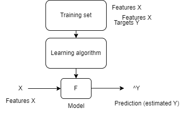
Our training see is define
We pass this training set to a learning algorithm
The learning output will be the model define which can predict data by inserting it some input
^Y is the prediction

We can by this way create the function like this :

W is the number of times used for the input X, it is the weight
B is the biais

It is the function to predict a line , here it is a linear way, which is easier than curve for prediction.

Let's illustrate this, by using to code :

We will use numpy to create or model and display to plot with matplotlib.

Then will create the training for our data by doing this :

 import numpy as np
import matplotlib.pyplot as plt

# x_train is the input variable (size in 1000 square feet)
# y_train is the target (price in 1000s of dollars)
x_train = np.array([1.0, 2.0])
y_train = np.array([300.0, 500.0])
print(f"x_train = {x_train}")
print(f"y_train = {y_train}")

You will use m to denote the number of training examples. Numpy arrays have a .shape parameter. x_train.shape returns a python tuple with an entry for each dimension. x_train.shape[0] is the length of the array and number of examples as shown below.

 # m is the number of training examples
print(f"x_train.shape: {x_train.shape}")
m = x_train.shape[0]
print(f"Number of training examples is: {m}")

# m is the number of training examples
m = len(x_train)
print(f"Number of training examples is: {m}")

Then we can plot our data using our lib :

 # Plot the data points
plt.scatter(x_train, y_train, marker='x', c='r')
# Set the title
plt.title("Housing Prices")
# Set the y-axis label
plt.ylabel('Price (in 1000s of dollars)')
# Set the x-axis label
plt.xlabel('Size (1000 sqft)')
plt.show()

The plot is defined, we can now define our function which will compute our model and return the output :

 def compute_model_output(x, w, b):
    """
    Computes the prediction of a linear model
    Args:
      x (ndarray (m,)): Data, m examples 
      w,b (scalar)    : model parameters  
    Returns
      y (ndarray (m,)): target values
    """
    m = x.shape[0]
    f_wb = np.zeros(m)
    for i in range(m):
        f_wb[i] = w * x[i] + b
        
    return f_wb

We are applying our function : 𝑓𝑤,𝑏(𝑥(𝑖)) where we can write :

for 𝑥(0) , f_wb = w * x[0] + b
for 𝑥(1) , f_wb = w * x[1] + b

Now lets add our function and compile it :

 tmp_f_wb = compute_model_output(x_train, w, b,)

# Plot our model prediction
plt.plot(x_train, tmp_f_wb, c='b',label='Our Prediction')

# Plot the data points
plt.scatter(x_train, y_train, marker='x', c='r',label='Actual Values')

# Set the title
plt.title("Housing Prices")
# Set the y-axis label
plt.ylabel('Price (in 1000s of dollars)')
# Set the x-axis label
plt.xlabel('Size (1000 sqft)')
plt.legend()
plt.show()

We should show the result of our chart like this :

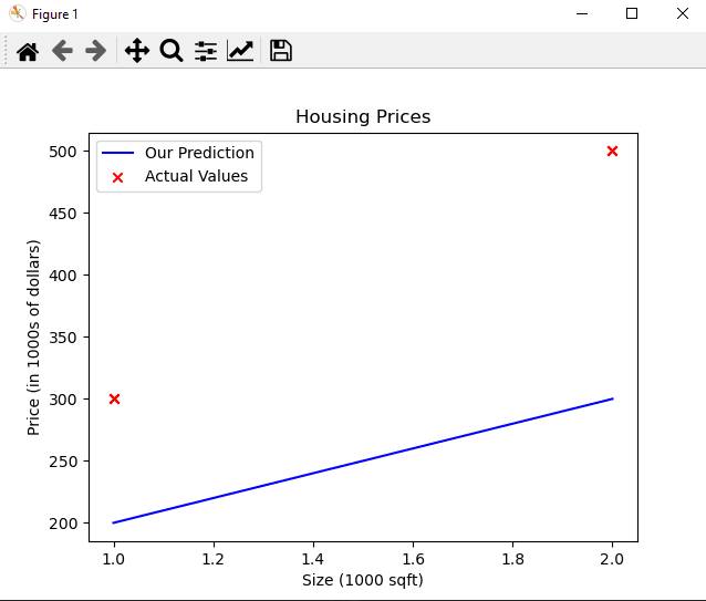
As you can see, setting $w = 100$ and $b = 100$ does not result in a line that fits our data.

Now that we have a model, we can use it to make prediction. Let's predict the price of a house with 1200 square feet. Since the units of 𝑥 are in 1000 feets, 𝑥 is 1.2.

 w = 200                         
b = 100    
x_i = 1.2
cost_1200sqft = w * x_i + b    

print(f"${cost_1200sqft:.0f} thousand dollars")

We should have as output :

 x_train = [1. 2.]
y_train = [300. 500.]
x_train.shape: (2,)
Number of training examples is: 2
Number of training examples is: 2
(x^(0), y^(0)) = (1.0, 300.0)
w: 100
b: 100
$340 thousand dollars

You can find the code there : Github - linear regression

Cost function

This function is telling, how well the model is doing, based on it we will be able to adjust to make him doing thing better.

Size in feet² (features)	Price in 1000$ (targets)
2104	400
1416	232
1534	315
...
3210	870

The model will use this data to train his model and use this formula :

w,b : are the parameters, used during training. Let's explain it, it is possible to have multiples graphs that we define with these parameters :

w	b	result	Explaining
0	1.5	F(x) = 0*X +1.5 = 1.5	The prediction is 1.5 (^y)
0.5	0	F(x) = 0.5*X +0	The slope is 0.5, as X will be our value to calculate, the value can variate
0.5	1	F(x) = 0.5*X +1	The slope is 0.5, as X will be our value to calculate can variate

When we define a graph and we saw a line passing closed to our value, or through like :

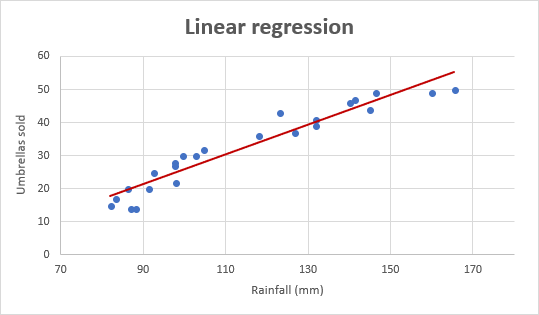
You can think of this to mean that the line defined by f is roughly passing through or somewhere close to the training examples as compared to other possible lines that are not as close to these points.

The question will be how can I find value for W and B ?

When we apply our formula :

Each dot on the graph is an interation called "i"
When can say that the formula become by the way :

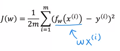
We will need to mesure how well a line fits the training data, to do that we create a "cost function": The cost function takes the prediction y hat and compares it to the target y by taking y hat minus y. We called this different : the error, where we're measuring how far off to prediction is from the target.

Let's computes the square of this error and we're going to want to compute this term for different training examples i in the training set. For example : we'll compute this squared error term.

We'll sum from i = 1,2,3 all the way up to m and remember that m is the** number of training items**, so if :

Notice that if we have more training examples m is larger and your cost function will calculate a bigger number.

We can predict this cost function like this :

In order to construct a cost function that is not affected by the size of the training set, we will use the average squared error as our measure of performance, instead of the total squared error. To achieve this, we will divide the total squared error by the number of training examples, represented by the variable m. This will ensure that the cost function remains consistent as the size of the training set changes.

The cost function that is commonly used in machine learning is typically divided by 2 times the number of training examples, represented by the variable m. This extra division by 2 is done for mathematical convenience during later calculations, however, it is not necessary for the function to work correctly. This cost function is referred to as J(w,b), also known as the squared error cost function, since it involves taking the square of the error terms. While different cost functions can be used for different applications in machine learning, the squared error cost function is a widely used and preferred choice for linear regression and other regression problems, as it has shown to give good results in many applications.

Finally our formula looks like :

We called this cost function : Squared error cost function.

So to recap :

Model :

parameters:

W,B. It will define the line of our graph and we want to define the correct value for W,B to make sure that this line fit ou is the more closer of our data. We need the cost function

Cost function :

The objectif, is to have J(w,b) the smaller as possible

We can simply our equations:

Model :

You can visualize this process as simplifying the original model on the left-hand side by removing the parameter b, or setting it to zero. This means that b no longer appears in the equation and f(x) is now simply represented by w times x.

parameters:

W,B. become W due to the fact that we removed "B"

Cost function :

When the parameter b is set to zero, the model becomes simpler, as it now has only one parameter, w. The goal of the model is to find the value for w that minimizes J(w). This simplification is visualized by the fact that the line defined by f(x) now passes through the origin. By looking at the graph of the model f(x) and the cost function J side by side, you can observe how the two are related. With the simplified model, it is important to note that while the estimated value of y depends on the value of the input x, the cost function J depends on the value of w, which controls the slope of the line defined by f(x).

Let's examine how the cost function varies when different values are chosen for the parameter w. To do this, we will plot the graphs of the model f(x) and the cost function J together. This will allow us to see how the two are related and how the cost function changes as the value of w changes.

First, it is important to note that when the parameter w is fixed, f(w) is only dependent on the input variable x. This means that the predicted value of y is determined by the value of x. On the other hand, the cost function J is dependent on the parameter w, which controls the slope of the line defined by f(w). In other words, the cost defined by J is affected by the value of w, as it is a function of w.

As an example, let's consider the value of w to be 1. For this choice, the function f(w) would result in a straight line with a slope of 1. To evaluate the cost function, we can calculate J(w=1) which is the cost of this particular value of w.

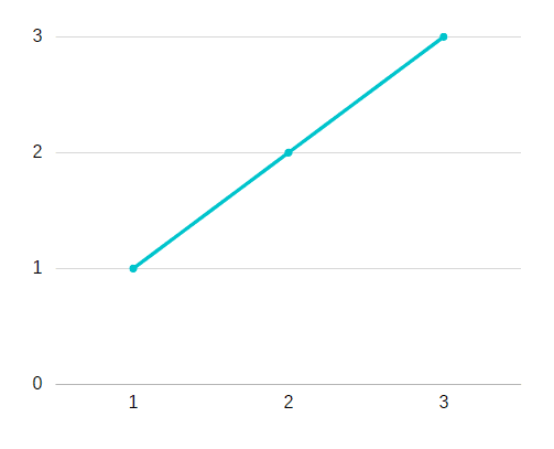
Lets take our function cost :

if W is equal to 1 we can supply it, because fw will equal to one
if X and Y are 1,2,3 together like on the graph, it cost 0 :

3. So for the 3 examples, the cost J is equal to 0.

To better understand how the cost function J(w) varies with the choice of w, we can plot J(w) as a function of w. Since J is a function of w, the horizontal axis will be labeled w instead of x, and the vertical axis will be labeled J instead of y.

For example, if we set w to be 1, we can calculate the corresponding cost J(w=1) which would be equal to 0, and plot it on the graph. We can also consider different values of w, such as negative values, zero, and positive values and observe how f(x) and J(w) change. For instance, when w=0.5, f(x) is now a line with a slope of 0.5 and we can calculate the cost J(w=0.5). This way, we can compare the different f(x) and J(w) corresponding to different values of w.

We are examining how the function f(x) and the cost function J(w) vary as the parameter w changes. The parameter w can take on a range of values, including negative, zero, and positive values. We can observe how these functions change by plotting them with different values of w. For instance, if we set w to 0.5, the function f(x) is a line with a slope of 0.5 and we can calculate the cost J(w=0.5). The cost function J(w) is measuring the difference between the predicted values by f(x) and the true values for each example in the dataset. This difference can be visualized as the height of the vertical line in the graph, representing the gap between the actual value of y and the value predicted by the function f(x) for a given value of x.

So the plot it :

We have the ligne and to difine the X value we will check the difference between or line and the objectif like :

(0.5-1)² + (1-2)² + (1.5-3)²
J(0.5) = 1/2m[(0.5-1)² + (1-2)² + (1.5-3)² ]
As we have 3 training example : m=3
(1/2*3)[3.5]
Where we can say 3.5/6 = 0.58 for the cost J

Note: w can be a negative value !

We can continue to evaluate the cost function J(w) for different values of the parameter w and plot them. By doing so, we can create a visual representation of how the cost function changes for different values of w. In this way, we can understand the shape of the cost function J(w) and how it behaves as we change the parameter value. This process gives us a way to determine the best value of the parameter w that minimizes the cost function J(w) and optimizes the model.

Given this, what is the method to choose the value of the parameter w that results in the function f fitting the data well? One approach is to choose the value of w that results in the smallest possible value of the cost function J(w). Since J(w) measures the squared errors between the predicted and actual values, minimizing this value will result in a better fitting model.

The main objective of linear regression is to determine the values of parameters such as w, or w and b that minimize the cost function J(w) . This is done so that the function f(x) generated by the model best approximates the true values in the given dataset.

Let's do it into a example using numpy :

You would like to develop a model that can predict the price of a house based on its size. To demonstrate this, let's use two sample data points: a house with 1000 square feet sold for $300,000, and a house with 2000 square feet sold for $500,000.

Consider this dataset :

Size (1000 feets)	Price (1000)
1	250
1.7	290
2.0	430
2.5	475
3.0	622
3.2	720

Consider to code this cost function, using python: 𝐽(𝑤,𝑏)=1/2𝑚∑𝑖=0𝑚−1(𝑓𝑤,𝑏(𝑥(𝑖))−𝑦(𝑖))²

 def compute_cost_function(x, y, w, b): 
    """
    Calculate the cost function for linear regression.
    The difference between the target (the value from our test) and the prediction is calculated and squared.
    Args:
      x (ndarray (m,)): Data, m examples 
      y (ndarray (m,)): target values
      w,b (scalar)    : model parameters  
    
    Returns
        total_cost (float): The cost of using w,b as the parameters for linear regression
               to fit the data points in x and y
    """
    # number of training examples
    m = x.shape[0] 
    
    cost_sum = 0 
    for i in range(m): 
        #f_wb is a prediction calculated
        f_wb = w * x[i] + b   
        cost = (f_wb - y[i]) ** 2  
        cost_sum = cost_sum + cost  
    total_cost = (1 / (2 * m)) * cost_sum  

    return total_cost

Now we have this cost function, we can initialize our data :

 #size in 1000 square feet
x_train = np.array([1.0, 1.7, 2.0, 2.5, 3.0, 3.2])
#price in 1000 square in dollar
y_train = np.array([250, 290, 475,  430, 622, 720,])


# Initialize model parameters
w = 0
b = 0

# Compute the cost
cost = compute_cost_function(x_train, y_train, w, b)
print("Initial cost: ", cost)


# Create a grid of (w,b) values
ws = np.linspace(-50, 50, 100)
bs = np.linspace(-100000, 100000, 100)
W, B = np.meshgrid(ws, bs)

# Compute the cost for all (w,b) values
Z = np.array([compute_cost_function(x_train, y_train, w_i, b_i) for w_i, b_i in zip(np.ravel(W), np.ravel(B))])

# Reshape the cost array to match the shape of (w,b)
Z = Z.reshape(W.shape)

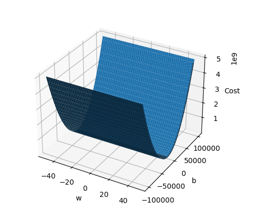
We have calculte the cost function for our price, we can change the value for W and B as mentionned previously. Let's visualize it into a plot :

 # Create a 3D plot
fig = plt.figure()
ax = fig.add_subplot(111, projection='3d')
ax.set_xlabel("w")
ax.set_ylabel("b")
ax.set_zlabel("Cost")
ax.plot_surface(W, B, Z)
plt.show()

Result :