Description

Self-Organizing Maps (SOM), also known as auto-adaptive maps, are an unsupervised clustering technique used in machine learning. SOM allows visualization and analysis of multidimensional data by projecting data points onto a two-dimensional neuron grid, called the SOM map. Each neuron on the SOM map represents a region in the multidimensional data space.

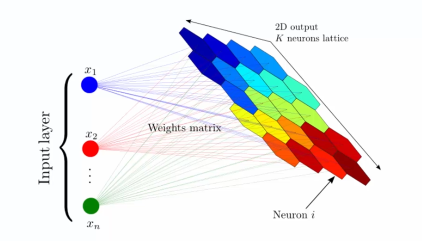
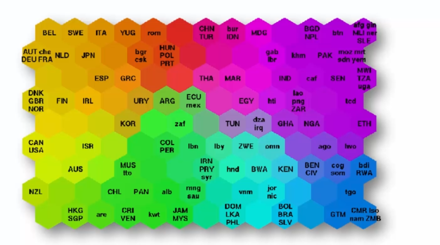
SOM is often used to identify patterns and relationships among data, particularly for exploratory data analysis. For example, using data on poverty levels in different countries, a SOM map can be used to visualize poverty levels and identify countries with similar levels of poverty.

Here is a simplified example: Suppose we have data on poverty levels in different countries. Using the SOM map, we could project this data onto a 5x5 neuron grid, where each neuron represents a cluster of countries with similar levels of poverty. The position of each country on the SOM map would be determined by its poverty characteristics, such as poverty rate, average income, etc.

By looking at the SOM map, we could identify regions of countries with similar levels of poverty. For example, countries in northern Africa could be grouped in one cluster, while European countries would be grouped in another. This would allow for quick visualization of poverty levels in different regions of the world and detecting interesting patterns in the data.

Here is an example of SOM visualization:

K-means

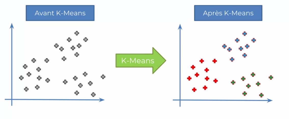
K-means is also an unsupervised clustering technique used in machine learning to identify groups of similar data points in a dataset. Unlike SOM, K-means does not project data onto a two-dimensional map but rather assigns each data point to one of the K pre-defined clusters.

How does it work?

The K-means algorithm is relatively simple. First, the user must specify the number of clusters K they want to use. Then, the algorithm selects K random points from the initial dataset to serve as initial cluster centers.

Next, each data point is assigned to the cluster closest to it in terms of Euclidean distance to the cluster centers. Once all points have been assigned to an initial cluster, the cluster centers are recalculated as the average of all points in each cluster. This process is repeated until the cluster centers converge to a stable position.

To give you a concrete example, suppose you have a dataset containing information on per capita income and poverty rate in different countries. You could use the K-means algorithm to group these countries into different clusters based on their poverty level.

For instance:

1. Choosing K clusters: First, we need to determine the number of clusters we want to create. This can be decided based on our objective or knowledge of the application domain. For example, if we are trying to segment customers of a company into distinct groups, we might choose K = 3 to identify high, medium, and low-income customers.

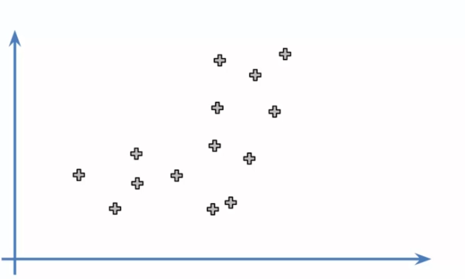
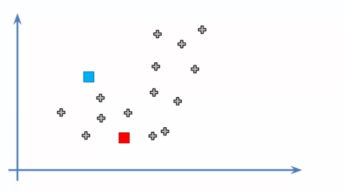
2. Initializing centroids: We now need to choose K random points in the dataset to serve as initial centroids. These centroids represent the centers of each cluster and will be adjusted as the algorithm iterates.

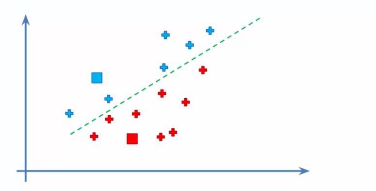
3. Assigning data to centroids: We assign each data point to its closest centroid. This creates K initial clusters and allows us to start seeing the different groups of data.

4. Recalculating centroids: We recalculate the centroids by taking the average of all data points associated with each cluster. This gives us a more precise position for each centroid and allows for readjustment of the clusters.

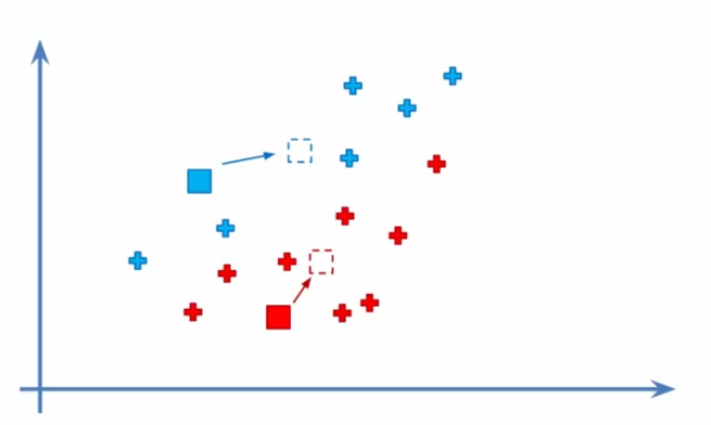
5. Reassigning data: We reassign each data point to its closest centroid based on the new calculated centroids. If any reassignments occur, we go back to step 4 to recalculate centroids and readjust clusters.

The initialization problem

One of the main challenges is the initial selection of centroids, which can significantly affect the final result. During the initial selection of centroids, it is possible to choose points that may not be representative of the dataset as a whole. This can lead to convergence towards suboptimal clusters. In some cases, this can even lead to divergence of the algorithm.

Let's take the example where k is equal to 3 clusters and set our centroids to create the 3 groups:

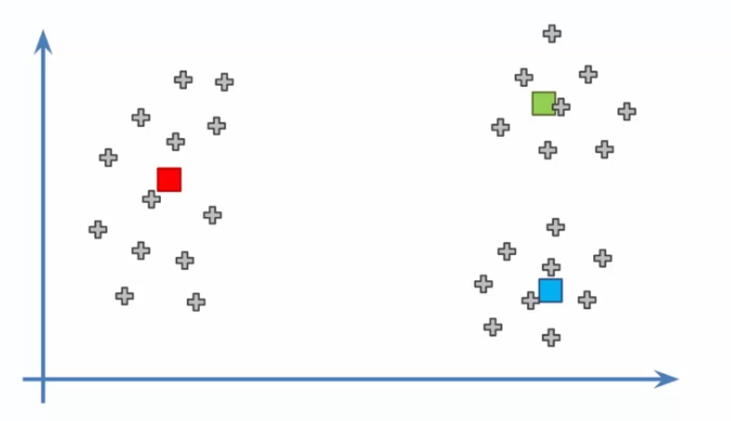
But can the algorithm converge? What would happen if we chose the initialization poorly?

Let's run our algorithm looking at the previous 5 steps:

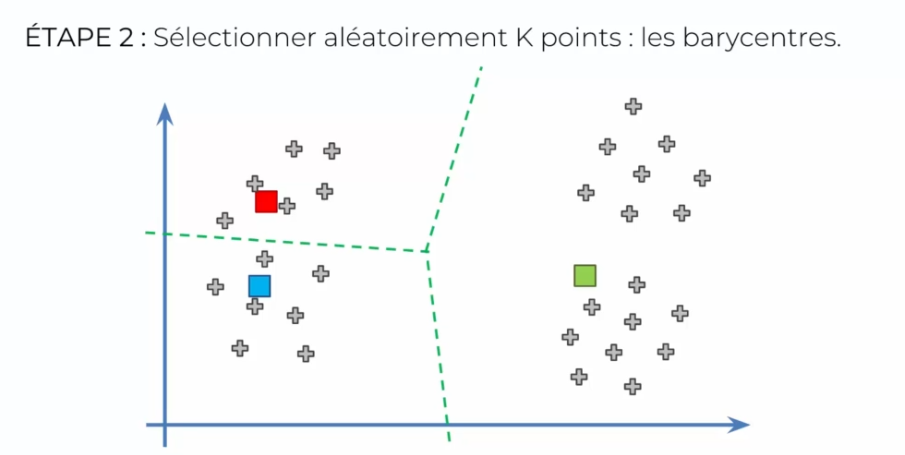
Then we move on to step 4 to move the centroids. Next, we arrive at step 5 which reassigns the points to the clusters. But we can see that nothing will change, so we are done! However, the clusters are now different:

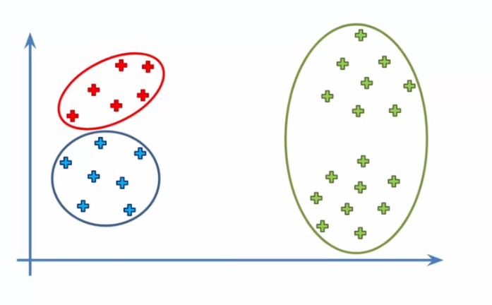
To avoid this problem, an improved method called K-means++ has been proposed. In the K-means++ algorithm, initial centroids are selected more intelligently. Instead of choosing random points, K-means++ uses a weighted selection method to select points that are further apart from each other. This method ensures that the initial centroids are well distributed in the dataset.

Furthermore, it is important to note that the K-means algorithm does not always converge to an optimal solution. Indeed, the convergence of the algorithm depends on the initial points and the nature of the data. In some cases, the algorithm may converge to a local minimum rather than a global minimum, which can give different results each time the algorithm is run.

Choosing the right number of clusters

Choosing the right number of clusters for the K-means algorithm is crucial to obtain relevant results. It is important to find the optimal number of clusters so that the algorithm can identify significant groups in the data. Here are some common methods for determining the number of clusters:

1. The elbow method: This method involves plotting the sum of squared distances of points to their centroid as a function of the number of clusters. We look for the point where the curve begins to have a slower decrease, like an elbow. This can help us identify the optimal number of clusters to use.

2. The silhouette method: This method involves evaluating the quality of the cluster partition. It calculates the average distance between each point and the other points in its cluster, then the average distance between each point and the closest neighboring cluster points. Then it calculates a silhouette measure for each point. The overall silhouette score is calculated by taking the average of silhouettes for all data points. A silhouette score close to 1 indicates well-grouped points, while a score close to 0 indicates poorly-grouped points.

3. The cross-validation method: This method involves splitting the data into two distinct sets, one for training and the other for validation. We use the training set to run K-means with different numbers of clusters, then evaluate the results on the validation set using a cluster quality measure, such as intra-cluster distance or explained variance.

Prompt

It is important to note that determining the optimal number of clusters is often subjective and depends on the application and user experience. In general, it is preferable to use multiple methods to evaluate different aspects of cluster quality and examine the results qualitatively and quantitatively.

SOM Learning

SOM learning is based on a neural network organized in a 2D grid of nodes, each node being associated with a weight vector representing its position in the data space. During the learning phase, the weights of each node are adjusted so that it can represent a region of the data space.

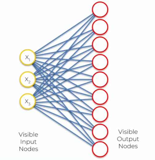
The learning process begins by initializing the weights of the nodes with random values. Then, for each input, the closest node is identified using a distance measure (e.g., Euclidean distance). This node is called the Best Matching Unit (BMU). The weights of the BMU and its neighbors are then adjusted to move closer to the input using a weight update rule based on the distance.

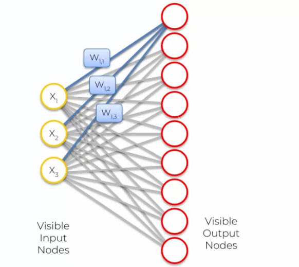
This weight update of the nodes leads to the formation of a self-organizing map that presents a topology similar to that of the input data. Nodes that are close in the map have similar weights, allowing for the visualization of the underlying structure of the data.

• Node1: (W1,1, W1,2, W1,3) because we have three inputs!
• Node2: (W2,1, W2,2, W2,3) because we have three inputs!
• ...

But why do we change this way of doing things? Because we create a competition between the output neurons. We pass through each neuron to determine which neuron is closest to the output, so we obtain the distance.

• Node1 : Distance = 1.2
• Node2: Distance = 0.8
• ...

Prompt

We have the distance for each neuron which corresponds between the input and output. The shortest distance is selected, and the winning neuron is called the Best Matching Unit (BMU). The next step is to adjust the weights so that the BMU is closest to our input. We will get an adaptation where we pull the output neuron towards the input:

We have a continuous adaptation of the map. But how does this work? Let's take the example of 5 BMUs colored by different colors:

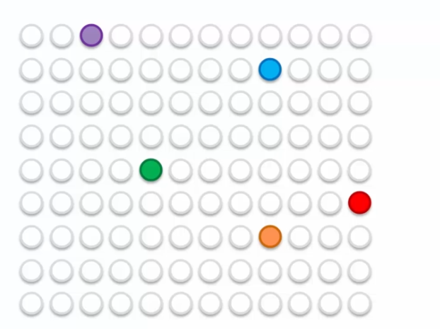
In the example, we have five BMUs colored in different colors. Neurons are updated to move closer to the closest lines as well as their influence circle. Each BMU pulls neurons towards it to reach a balance at the end of each epoch. The process repeats until the self-organizing map is stabilized.

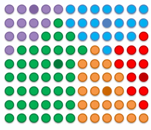
The process becomes more and more accurate with each epoch as the influence radius of the BMUs is reduced. This process allows data to be grouped into clusters and visualize the underlying structure of the data. The self-organizing map can be used to perform tasks such as complex data classification and visualization.

Conclusion

SOMs retain the topology of the training set by creating a self-organizing map that preserves the topological relationships between the data. This feature is important because it allows correlations to be visualized that may be difficult to identify otherwise.

Unlike supervised learning techniques, SOMs do not require specific targets as they perform data categorization without supervision. SOMs use competition between the output neurons to determine the BMU closest to the input and adjust the weights accordingly.

It is also important to note that SOMs do not have lateral connections between the output nodes. This means that each node is independent and only processes the inputs presented to it. This feature allows for large-scale data processing with high efficiency and low complexity.