Reinforcement Learning

In Machine Learning, we define an environment in which our artificial intelligence (AI) will take actions, learn, and evolve. Thus, our "agent," which will be our AI, takes actions and receives rewards (and states) based on these actions.

The goal of Machine Learning is to enable the agent to learn to take the best possible actions in this environment to optimize its long-term rewards. This requires active exploration of the environment by the agent to discover the actions that will maximize its long-term rewards.

Thus, the agent will know, in an environment, how an action can earn it a reward and which actions will not. As in real life, when we perform actions, we are rewarded for successful actions, but we also learn from our mistakes to progress towards our goals.

The Bellman equation is indeed a fundamental principle of reinforcement learning. It formalizes the calculation of the expected reward for a given action in a given state of the environment.

The Bellman equation

Let's start:

• S: State
• S': Final state
• A: Action
• R: Reward
• Y: Discount

Let's take the example of an agent who needs to get to an endpoint:

When an agent performs an action (A) in a state (S), it receives a reward (R) and ends up in a new state (S'). The agent's goal is to maximize the sum of the rewards it receives throughout its actions, taking into account the fact that future rewards are discounted by a factor Y. Thus, the agent must learn to choose the best actions in each state to maximize the sum of the rewards it will receive until it reaches the final state (S').

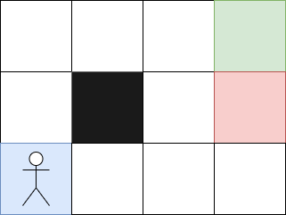
Here, if the agent goes to the red square, it will receive a penalty, and if it arrives at the green square, it will receive a reward. The black square cannot be crossed. At first, the agent will take random actions because it will not know what to do. Then, it will gradually learn which actions to take to reach the endpoint.

Each step to reach the final square will have a value of 1. These values will then allow the agent to reproduce the path indefinitely.

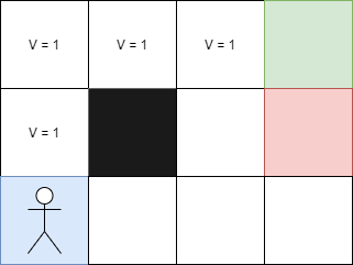
But what happens if the agent moves to a different starting position, such as the top left? In this case, the approach does not work particularly well. To remedy this, the Bellman equation is used:

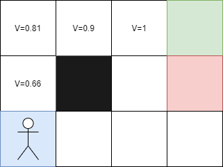
In our previous problem, each square corresponds to a state. So, if I take the next square, what will its value be?

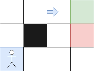
Consider the following example: the reward for going right is +1 because it corresponds to the arrival. Since we are at the end, there is no discount to apply, and the value of this state is therefore V = 1.

Now, let's take the left cell: the reward for going right is 0 because this white cell does not give a reward. We apply the discount factor Y of 0.9 (arbitrary value chosen here) to the value of the next state, which is 1, and we get Y * V of the next cell, which is 0.9 * 1 = 0.9. Thus, the value of this state is V = 0.9.

Let's continue with the left cell: if we go right, we will not get a reward because it is a white cell. We apply the discount factor Y of 0.9 to the value of the next state to the right, which is 0.9, and we get Y * V of the next cell, which is 0.9 * 0.9 = 0.81. Thus, the value of this state is V = 0.81.

And so on to calculate the value of each state using the Bellman equation, which allows to calculate the value of a state based on the reward obtained for the action taken in that state and the value of the following states weighted by the discount factor Y.

Here is a spelling correction and a proposal for a clearer and easier-to-understand structure regarding the Bellman equation:

Thus, the further away from the arrival, the more the value of V decreases, which is normal. Now, each cell has a higher value if it is close to the arrival, so I can start on any cell.

But what is the value of the cell to the left of the red cell? Since it is impossible to go left from the red cell, we have three possible directions. If I go up, I will have a V value of 0.9 because we know that the top cell has a value of 1.

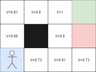
The Bellman equation allows to calculate the value of a state based on the reward obtained for the action taken in that state and the value of the following states weighted by the discount factor Y. The further the agent moves away from the arrival, the more the value of the state decreases, and conversely, the closer the agent gets to the arrival, the more the value of the state increases. Thus, by using this equation, we can calculate the value of each state and determine the best action to take in each state to maximize the rewards obtained.

Plan and Markov

The plan consists of replacing the values of the cells with arrows to obtain the optimal path. To do this, we evaluate the direction to take from a cell by looking at the adjacent cell that has the highest value. This allows us to determine the directions resulting from the Bellman equation and obtain a clear path for our agent.

However, does this suffice to define artificial intelligence? Not at all! We must talk about the processes involved.

However, is that enough to define artificial intelligence? Not at all! We must talk about the processes involved.

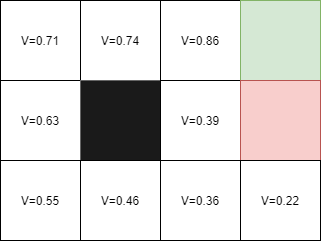
In a deterministic process, if the agent moves upwards, it will have a 100% probability of arriving there because it is heading straight there. However, in a non-deterministic process, there is a difference between what we want and what actually happens. In general, we cannot predict with 100% certainty what will happen.

The Markov process is a stochastic process in which the future depends only on the present state and not on past states. Thus, all past actions have no influence on the current state. In the Markov decision process (MDP), the agent cannot fully control the outcome of its decision, but it can choose the decision to take using a Markov process to determine the most likely direction to follow.

To integrate this factor with the Bellman equation:

OR (more complicated but equivalent)

In the Bellman equation, we use the discount factor Y to weight the values of future states based on their probability of occurrence. Thus, we can take into account the probability of reaching a given final state by adding action probabilities. For example, if we have a probability that an action will lead us to the red square, we need to take this probability into account in our decision scheme.

This brings us to asking the right questions. Given that we have a probability that a direction might make us fall on the red square, our decision scheme must take this probability into account to avoid potential losses. Thus, the Markov decision process (MDP) is used to take into account the probabilities of occurrence and potential risks in decision-making for an agent using the Markov process:

Life penalty

It is important to remember that in the context of reinforcement learning, the AI receives a penalty at the end of its journey. However, in reality, we should rather add small rewards at each step to help the AI navigate the environment. For example, in the case of a maze, the agent will accumulate rewards at each move, which will help it progress towards the exit. In this case, the rewards will be -0.04 as the goal of the AI is to exit the maze as quickly as possible. Thus, by adding rewards at each step, we can help the AI find the best path to the exit.

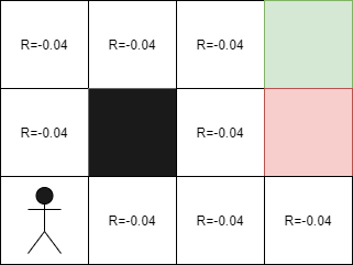
When we add negative rewards at each step, our goal is to "squeeze" the AI to find the fastest path to the goal. However, what would happen if we used larger negative rewards?

• When R(s) = 0, we avoid the red square and even take the risk of hitting walls to avoid going directly up, and instead go to the right or left.

• When R(s) = -0.04, we no longer take the time to hit the walls, but we still try to avoid the red square as much as possible.

• When R(s) = -0.5, we try to go to the starting square by any means necessary, even if it means taking the risk of passing near the red square.

• When R(s) = -2.0, our goal is to finish the game as quickly as possible, as -2 is a greater penalty than that of the red square. Thus, the least worst may be to fall into the red square to finish the game more quickly.

By using larger negative rewards, we push the AI to take greater risks to reach its goal as quickly as possible. This can have advantages and disadvantages, depending on the goal of the AI and the constraints of the problem to be solved.

Qlearning intuition

Here, we measure a quality when we are in a state (S). Thus:

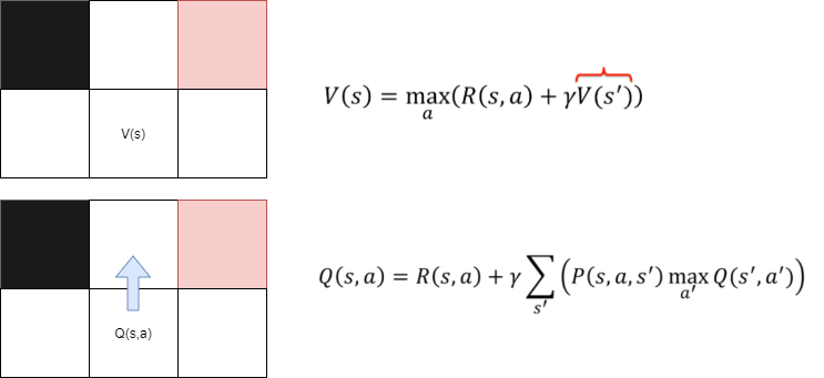
To calculate the optimal value of a square, we use the same method as before with the Bellman equation. We calculate the weighted average of arriving on a square to find the best possible action.

Thus, the value of Q(s,a) is equal to the value of V(s), where V(s) is the maximum possible for square s. Using Q(s,a), we can calculate the best possible action for state s. This depends on the value of V(s') for future states s'. Thus, we can say that the value of Q(s,a) depends on the value of V(s') to find the best action to take.

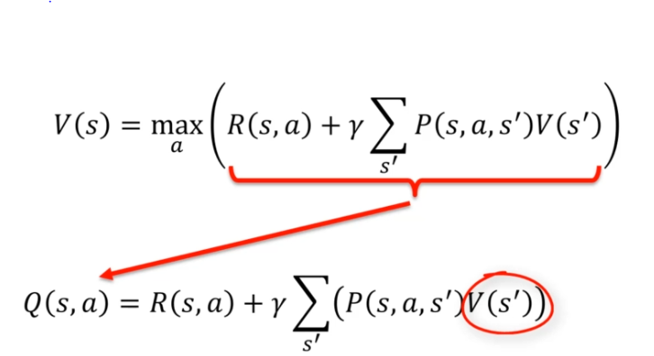
Temporal Difference

Remembering the deterministic and non-deterministic methods, we can take the example of the last square, whose value was:

• Deterministic: V = 1, because we had a reward of +1 to reach this square.
• Non-deterministic: V = 0.86, with a probability of 80% of reaching the final square. To find the previous value of V = 0.86, we need to calculate the value of V = 0.39 and so on. This can lead us to fall into a calculation loop to determine the values of the states.

By using our new value update function, the temporal difference, we can solve this problem by updating the values of states based on the difference between current and future values. Using this method, we can quickly calculate the values of states without needing to calculate all previous values. This allows us to save time and energy in the reinforcement learning process.

OR

Let's take an example, imagine that in our environment we start on this square:

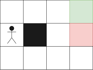
Our AI has already performed calculations to find the optimal values for each state. For our first attempt, the initial values for each state will be random values.

Before taking an action, we calculate the value of Q(s,a) to find the best possible action for the current state s. Once the action has been taken, we use temporal difference to update the values of the states.

After taking an action, we can apply:

After taking an action in state S, we receive a reward. Using this reward, we can calculate the temporal difference, which is the difference between the future state after taking the action and the current state before taking the action. This temporal difference can be written as:

When the temporal difference is 0, this means that the value of the current state is equal to the sum of the values of the future states weighted by their probabilities and rewards, as defined by the Bellman equation. This may be the case if our AI has been successfully trained for some time, but it will not always be the case at the beginning.

If we encounter a situation where we get a value we did not expect (for example, a random event of 10%), we do not want to lose the previous value by immediately updating the value of the state. To avoid this, we use a time coefficient, which we multiply by alpha (a parameter between 0 and 1). This allows us to update the value of the state slowly, giving less importance to the random value, while still keeping track of the previous value. This makes the reinforcement learning process more robust and effective.

If we combine everything:

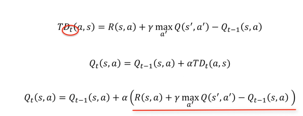
When using the time coefficient alpha, we need to find a balance between exploiting the previous values and updating the new values. If we take an alpha of 0, the temporal expression is cancelled out, and the agent will not be able to learn anything. If we take an alpha of 1, the previous values of Qt-1(s, a) are completely cancelled out, and the agent focuses only on the new values.

Therefore, we need to choose an alpha that lies between these two extremes, in order to maintain a memory of the past and present. The goal is to make the value of Q as stable as possible, while keeping in mind that the environment can change and the value of Q may need to be re-evaluated.

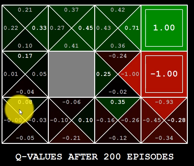
An example of Q-learning could be:

Deep learning intuition

In the previous example, our agent had constant rewards for each action, which allowed the agent to assign values to each box and develop a strategy to reach the endpoint.

However, in more complex cases such as autonomous driving, there may be many unforeseen factors such as pedestrians, animals, etc. It would be impossible to create a state for every possibility.

To solve this problem, we can create states with two dimensions in the case of our maze, for example (X1, X2). This method is called Deep Q-Learning, and it allows our agent to learn to navigate in a more complex environment by creating abstract states that encapsulate multiple real states. In other words, our agent can learn to identify similar situations and make decisions accordingly, even if it has never encountered an exactly identical situation.

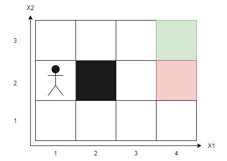
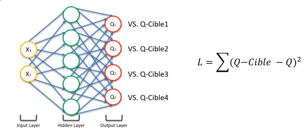
In Deep Q-Learning, there is no longer the notion of before and after. Here, the neural network will output 4 predictions for Q(s,a): Q1, Q2, Q3, Q4. At the beginning, we have no values for these predictions. To do this, we will retrieve the values we have already received through the Bellman algorithm. Thus, we can compare our values with the Q-targets. We will then calculate a cost function via these Q-targets. We will then do our backpropagation, which will update our weights on our Hidden layer.

Experience replay

When using Deep Q-Learning, the neural network can be unstable and not easily convergent. Additionally, it must process a large amount of information at once. To remedy these issues, the experience replay technique is used. This method involves replaying past experiences randomly so that the agent can learn from similar situations encountered in the past.

Experience replay is a technique used in reinforcement learning to improve the stability and performance of deep Q-learning algorithms. This technique involves storing all past experiences (environment observations, actions taken by the agent, rewards obtained, and next states) in a buffer memory called "replay buffer".

Instead of updating the neural network weights for every new experience, we will randomly select past experiences from the replay buffer and use them to train the network. This technique prevents the neural network from being biased by specific experiences and ensures diversity of the training data.

Experience replay allows for effective reuse of training data and minimizes the training time of the neural network. Indeed, by reusing past experiences, we limit the number of updates required to achieve optimal performance.

Action selection strategy

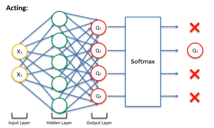
The idea of the function is to find a balance between exploration and exploitation. In general, we have multiple possible values for an action, and we will choose the highest one. However, this can pose problems because new events could completely change the situation. In the case of exploration, we are precisely looking for new solutions that could emerge. Thus, there are several action selection strategies:

• ε-greedy : Choose a value ε between 0 and 1, which represents a percentage. For example, if ε = 10%, then 10% of the time, we make a totally random decision, and the rest of the time, we take the best possible decision. Thus, 10% of the time, we do exploration (testing possible novelties), and 90% of the time, we rely on what we have learned (exploitation).

• ε-soft(1-ε): This strategy is exactly the same as the previous one, but we invert the value of ε. Thus, 90% of the time, we take the best possible decision, and 10% of the time, we do exploration.

• Softmax: For each output neuron, we have a value z that represents the quality of the corresponding action. We then apply an exponential function to each of these values, and normalize the result to have a sum equal to 1. This gives us a probability for each possible action. We then randomly choose an action, following these probabilities. This strategy is interesting because it allows us to choose actions in a less deterministic way than the previous strategies, while still maintaining some coherence.

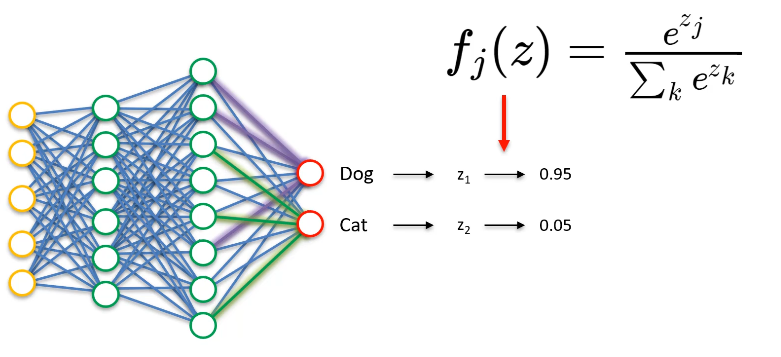
So we have the concept of exploration vs. exploitation, that is, knowing which of these two concepts we should use more often. Let's take an example:

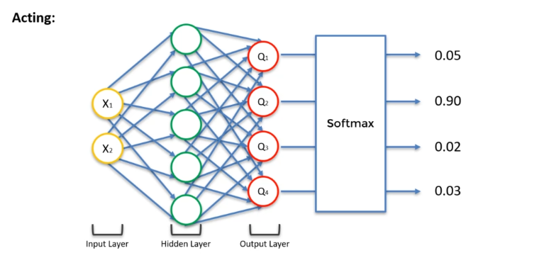
The answer here doesn't say that Q2 will necessarily be the right value, but that there is a 90% chance that it is. Q1 could also be the right value. In other words, each action has a percentage chance of being chosen. Thus, there is a balance between exploration and exploitation. At the beginning, we need to do a lot of exploration to determine the most probable Q value.

Eligibility trace

The eligibility trace is a reinforcement learning method that measures the contribution of each action in obtaining a reward. It is used to optimize learning and decision-making in reinforcement systems.

The eligibility trace is calculated by assigning an eligibility value to each step or action, which represents the contribution of that action to obtaining the reward. This value is updated at each step based on the importance of the action in obtaining the reward.

The eligibility trace takes into account the history of actions and rewards to optimize decision-making. It weights actions based on their importance in obtaining the reward and favors actions that have contributed the most to obtaining the reward.

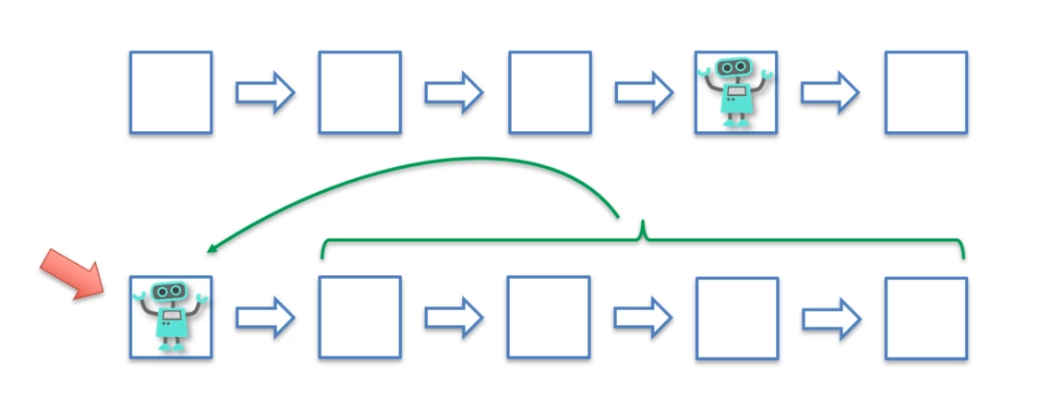
In the first case, the robot moves from square to square based on the rewards it receives at each step. In the second case, the robot tests different combinations of squares and evaluates whether they are beneficial or not.

In the first case, the robot simply acquires rewards as it goes along without taking enough step back to optimize its choices. In the second case, the robot analyzes the combinations of steps that have worked well, but also those that have not worked well in order to correct its choices to reach the best possible step. This analysis is made possible by the eligibility trace, which allows us to trace the steps that led to the reward obtained. Thus, the robot can easily correct its errors and find the best step.

A3C : Asynchronous Advantage Actor-Critic

The A3C (Asynchronous Advantage Actor-Critic) is one of the most powerful algorithms in the field of artificial intelligence. It is a reinforcement learning algorithm developed by Google in 2016 that is more efficient than previous algorithms and allows for a faster learning phase.

The A3C combines several reinforcement learning techniques, including actor-critic and asynchronous advantage.

Actor-critic

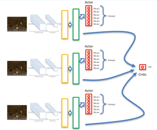
In the Actor-critic algorithm, a second output is added to the neural network. The first output is the Q-value representation, which is handled by the actor, and the second output is the V-value, which represents the value of a particular state and is handled by the critic.

The role of the actor is to choose the actions to be taken, while the role of the critic is to evaluate the quality of those actions. By combining the two outputs, the Actor-critic algorithm can both learn to choose the best possible actions and evaluate the quality of those actions in real-time.

The Actor-Critic algorithm is commonly used in reinforcement learning and has helped to solve many complex problems in artificial intelligence. By combining the advantages of the actor and the critic, it allows for better learning performance and more effective decision-making.

Asynchronous

Instead of using a single agent, the method is to use two agents that start from different points. This increases the number of explorations and reduces the risk of an agent getting stuck. The agents can then learn from each other through their explorations and share the critic value. This value V is associated with a shared neural network, which is made available to the agents' neural networks.

Thus, by using this method, we have N agents, each with their own neural network, as well as a shared neural network. This approach optimizes reinforcement learning and achieves better performance by using collaboration between agents.

Avantage

When the function V appears in the algorithm, it is necessary to give it a notion of cost. This is where the value of Policy Loss comes in, which allows quantifying how good or bad an action is.

First of all, it is important to recall the advantage formula: A = Q(s,a) - V(s). Then, we can explain the cost values:

Value Loss: This cost function allows comparing the estimated Q value to the Q value obtained by applying the Bellman method.

Policy Loss: This cost function allows quantifying how good or bad an action is. If the Q value is greater than 2, it means that the chosen action is better than expected. Conversely, if the Q value is less than 1, it means that the chosen action is not good.

These cost functions are then backpropagated into the neural networks to improve the critical value of V as well as the value of s and a, in order to maximize the advantage of the equation. This allows optimizing decision making and improving the performance of the reinforcement learning algorithm.

Long Short-Term Memory (LSTM)

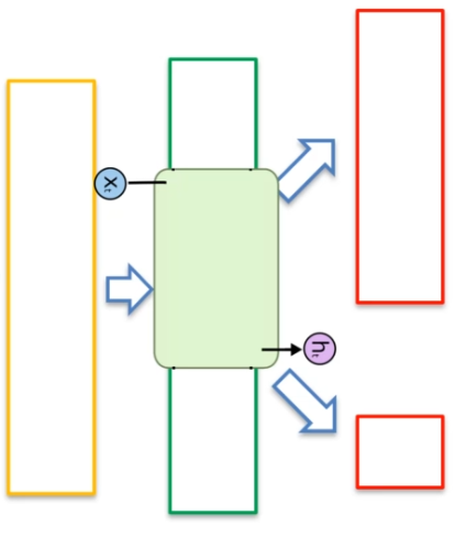
An important modification was made at the level of the hidden layer by adding an LSTM layer. This layer allows the neural network to have a memory, allowing it to remember what happened previously. When an image is input to the network, it can now remember past events and memories of previous states.

By using an LSTM layer, the neural network can improve its performance in reinforcement learning by taking into account the previous states. This allows the neural network to better understand the sequences of actions and to make more effective decisions based on past events. The long-term memory thus allows the neural network to better model the context and improve its ability to make precise decisions based on the current situation.

How does it work?

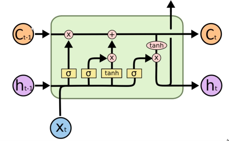
In an LSTM neural network, we have an input Xt that corresponds to the previous layer and an output Ht that corresponds to the next layer (upward arrow in the diagram). In addition to these inputs and outputs, we have two other inputs:

• Ht-1: This input allows the neural network to remember the previous step and learn from it. It is a value that is reused for the next step.
• Ct-1: This input corresponds to the memory of the previous step. It is a persistent information that allows the neural network to remember past events.

The LSTM neural network also has two outputs:

• Ct: This output corresponds to the output memory. It allows the neural network to store information for later use.
• Ht: This output is reused for the next step of the neural network. It allows the neural network to remember the previous state and use this information to make more precise decisions based on the current context.

By using these inputs and outputs, the LSTM neural network can improve its ability to take into account the history of past events and make more precise decisions based on the current context.