What's is this ?
Machine learning is a powerful tool that can be used to make predictions and decisions based on data. However, as with any tool, it is important to use it correctly in order to get the best results. In this article, we will explore two common problems that can occur when using machine learning algorithms: overfitting and underfitting.
Overfitting and underfitting
First, let's take a look at overfitting. Overfitting occurs when a model is too complex for the data it is trying to fit. This can happen when there are too many features or when the model is too flexible. The result is that the model fits the training data perfectly, but performs poorly on new data.
To illustrate this concept, let's consider an example of predicting housing prices with linear regression. Suppose our data looks like this:
| Size of House (x) | Price (y) |
|---|---|
| 1000 | 200,000 |
| 1200 | 250,000 |
| 1400 | 300,000 |
| 1600 | 350,000 |
| 1800 | 400,000 |
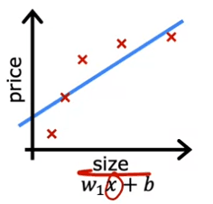
One thing we could do is fit a linear function to this data. If we do that, we get a straight line fit to the data that looks like this:
y = 200,000 + 0.2x
But this isn't a very good model. Looking at the data, it seems pretty clear that as the size of the house increases, the housing price flattens out. This algorithm does not fit the training data very well. The technical term for this is that the model is underfitting the training data. Another term is that the algorithm has high bias.
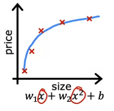
Now, let's look at a second variation of a model, which is if we insert a quadratic function into the data with two features, x and x^2. Then when we fit the parameters W1 and W2, we can get a curve that fits the data somewhat better. Maybe it looks like this:
y = 200,000 + 0.2x + 0.001x^2
Also, if we were to get a new house that's not in this set of five training examples, this model would probably do quite well on that new house. If you're real estate agents, the idea that you want your learning algorithm to do well, even on examples that are not on the training set, that's called generalization. Technically we say that you want your learning algorithm to generalize well, which means to make good predictions even on brand new examples that it has never seen before. These quadratic models seem to fit the training set not perfectly, but pretty well. I think it would generalize well to new examples.
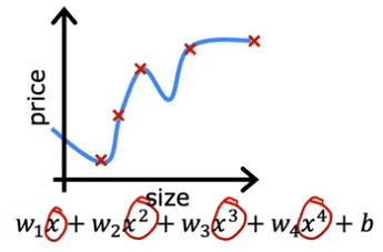
Now let's look at the other extreme. What if we were to fit a fourth-order polynomial to the data? You have x, x^2, x^3, and x^4 all as features. With this fourth-order polynomial, we can actually fit the curve that passes through all five of the training examples. But this is clearly overfitting the data. This model is too complex and flexible for the data and it is likely to perform poorly on new data.
In order to avoid overfitting, we can use techniques such as regularization. Regularization is a technique that helps us minimize the overfitting problem and get our learning algorithms to work much better.
It is important to keep in mind that overfitting and underfitting are not always easy to recognize, and that sometimes it may require some experimentation to find the correct balance between underfitting and overfitting. This is why it is important to also check the performance of the model on the test set, which is not used for training, to see how well the model generalizes to new unseen examples.
Example
Let's import our dependencies, using a librairy that you can find into our github :
 import matplotlib.pyplot as plt
from ipywidgets import Output
from plt_overfit import overfit_example, output

plt.close("all")
display(output)
ofit = overfit_example(False)
The output of this code will be:
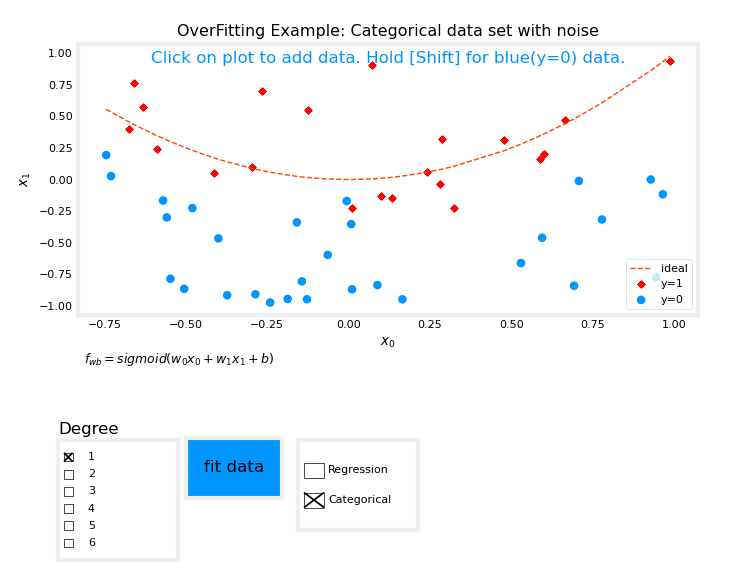
The above plot allows you to switch between Regression and Categorization examples, add data, select the degree of the model, and fit the model to the data.
You should try fitting the data with degree = 1 and noting the 'underfitting,' fitting the data with degree = 6 and noting the 'overfitting,' and tuning the degree to get the 'best fit.'
Adding data such as extreme examples can increase overfitting, while nominal examples can reduce it. The 'ideal' curves represent the generator model to which noise was added to create the data set, and the 'fit' function uses a method other than pure gradient descent for improved speed and can be used on smaller data sets.
How to address ?
Overfitting is a common problem when working with machine learning algorithms. It occurs when a model is trained too well on the training data, and as a result, it performs poorly on new, unseen data. In this article, we will discuss ways to address overfitting and make your model more robust.
Collect more training data
One way to address overfitting is to collect more training data. As the number of training examples increases, the learning algorithm will learn to fit a function that is less wiggly, and thus, less prone to overfitting. For example, if we are trying to predict house prices, and we have a limited number of data points, we can gather more data on sizes and prices of houses to make our model more robust. However, getting more data may not always be an option, and in such cases, we can explore other options.
Fewer features
Another way to address overfitting is to use fewer features. In some cases, overfitting can occur when there are too many features and not enough data. In such cases, we can select a subset of the most useful features, and use only that to train our model. This process is known as feature selection. It is important to note that feature selection may lead to throwing away some of the information that you have about the houses.
Regularization
The third option for reducing overfitting is regularization. Regularization is a technique that encourages the learning algorithm to shrink the values of the parameters without necessarily eliminating them. This makes the model less complex and less prone to overfitting. In the next section, we will discuss regularization in more depth and see how it can be used to improve our models.
In summary, overfitting is a common problem when working with machine learning algorithms, and it can be addressed by collecting more data, using fewer features, or regularization. Each of these options has its own advantages and disadvantages, and it is essential to choose the one that best suits your problem. In later courses, we will also discuss more advanced techniques for addressing overfitting, such as cross-validation, and early stopping.
How it works with cost function ?
Regularization is a technique that is used to address overfitting in machine learning algorithms. It works by adding a penalty term to the cost function, which discourages the model from having large parameter values. In this article, we will discuss how regularization can be applied to your learning algorithm to make your model more robust.
First, let's recall an example from the previous section, in which we saw that if you fit a quadratic function to data, it gives a good fit. But if you fit a very high-order polynomial, you end up with a curve that overfits the data. To address this issue, we can modify the cost function and add a term that penalizes the model if the parameters W3 and W4 are large. For example, we can add 1000 times W3 squared plus 1000 times W4 squared to the cost function. This modified cost function will encourage the model to have smaller values for W3 and W4, which is equivalent to having a simpler model with fewer features, and thus less prone to overfitting.
The idea behind regularization is to penalize all the parameters Wj, instead of just W3 and W4. This way, we don't have to know which features are the most important, and we can use all the features without worrying about overfitting. For example, if we have data with 100 features for each house, it may be hard to pick which features to include and which ones to exclude. So, let's build a model that uses all 100 features, and penalize all of them by adding a new term lambda times the sum of wj squared. This value lambda is called the regularization parameter, and it has to be chosen carefully.
In conclusion, regularization is a technique that can be used to address overfitting in machine learning algorithms. It works by adding a penalty term to the cost function, which discourages the model from having large parameter values. By convention, the regularization term is divided by 2m, which makes it easier to choose a good value for lambda, and it is also scale-invariant, meaning that the same value of lambda can be used regardless of the size of the training set. In later courses, we will also discuss more advanced techniques for regularization, such as L1 and L2 regularization.
Regularized linear regression
Linear regression is a commonly used method for modeling the relationship between a dependent variable and one or more independent variables. However, in some cases, the model may become overfit, meaning it fits the training data too well and may not perform well on new data. To avoid overfitting, we can add a regularization term to the cost function.
The cost function for regularized linear regression is a combination of the usual squared error cost function and an additional regularization term. The regularization term is controlled by a parameter, Lambda, and the goal is to find the parameters w and b that minimize the regularized cost function.
So let's define our formula :

Where: 𝑓𝐰,𝑏(𝐱(𝑖))=𝐰⋅𝐱(𝑖)+𝑏
We can imagine to implement it like this :
 def compute_cost_linear_reg(X, y, w, b, lambda_ = 1):
    """
    Computes the cost over all examples
    """

    m  = X.shape[0]
    n  = len(w)
    cost = 0.
    for i in range(m):
        f_wb_i = np.dot(X[i], w) + b
        cost = cost + (f_wb_i - y[i])**2
    cost = cost / (2 * m)

    reg_cost = 0
    for j in range(n):
        reg_cost += (w[j]**2)
    reg_cost = (lambda_/(2*m)) * reg_cost

    total_cost = cost + reg_cost
    return total_cost
Previously, we used gradient descent for the original cost function. However, now that we have added the regularization term, the updates for the parameters w and b are slightly different. The update for w is given by the following formula: w_j = w_j * (1 - Alpha * Lambda / m) - Alpha * (1/m) * term
where Alpha is a small positive number called the learning rate, m is the training set size, and term is a specific expression for the derivative of the cost function with respect to w_j. The update for b remains the same as before.
It is important to note that the regularization term only affects the update for w, not b. This is because the goal of regularization is to shrink the parameters, and in this case, we are trying to shrink the parameters w, but not b.
To implement gradient descent for regularized linear regression, the updates for w and b should be carried out simultaneously. The update for w should be performed for all values of j from 1 to n, and the update for b should be performed according to the previous formula.
So let's define our formula :

We can imagine to implement it like this :
 def compute_gradient_linear_reg(X, y, w, b, lambda_):
    """
    Computes the gradient for linear regression
    """
    m,n = X.shape           #(number of examples, number of features)
    dj_dw = np.zeros((n,))
    dj_db = 0.

    for i in range(m):
        err = (np.dot(X[i], w) + b) - y[i]
        for j in range(n):
            dj_dw[j] = dj_dw[j] + err * X[i, j]
        dj_db = dj_db + err
    dj_dw = dj_dw / m
    dj_db = dj_db / m

    for j in range(n):
        dj_dw[j] = dj_dw[j] + (lambda_/m) * w[j]
In summary, regularized linear regression is a method for avoiding overfitting in linear regression models. It is implemented by adding a regularization term to the cost function and updating the parameters using gradient descent. The updates for the parameters are slightly different than before, with the regularization term only affecting the updates for w, not b. This allows us to shrink the parameters w to improve the model's performance on new data.
Regularized logistic regression
In this section, we will be discussing regularized logistic regression and how to implement it using gradient descent. Logistic regression is a commonly used method for modeling the relationship between a dependent variable and one or more independent variables in classification problems. However, in some cases, the model may become overfit, meaning it fits the training data too well and may not perform well on new data. To avoid overfitting, we can add a regularization term to the cost function.
The cost function for regularized logistic regression is a combination of the usual logistic regression cost function and an additional regularization term. The regularization term is controlled by a parameter, Lambda, and the goal is to find the parameters w and b that minimize the regularized cost function.
So let's define our formula :

Where: 𝑓𝐰,𝑏(𝐱(𝑖))=𝑠𝑖𝑔𝑚𝑜𝑖𝑑(𝐰⋅𝐱(𝑖)+𝑏)
We can imagine to implement it like this :
 def compute_cost_logistic_reg(X, y, w, b, lambda_ = 1):
    """
    Computes the cost
    """

    m,n  = X.shape
    cost = 0.
    for i in range(m):
        z_i = np.dot(X[i], w) + b
        f_wb_i = sigmoid(z_i)
        cost +=  -y[i]*np.log(f_wb_i) - (1-y[i])*np.log(1-f_wb_i)

    cost = cost/m

    reg_cost = 0
    for j in range(n):
        reg_cost += (w[j]**2)
    reg_cost = (lambda_/(2*m)) * reg_cost

    total_cost = cost + reg_cost
    return total_cost
Just like regularized linear regression, the gradient descent update for regularized logistic regression will also look similar. The update for w is given by the following formula:
*w_j = w_j - Alpha * (1/m) * (term + (Lambda/m)w_j)
where Alpha is a small positive number called the learning rate, m is the training set size, and term is a specific expression for the derivative of the cost function with respect to w_j. The update for b remains the same as before.
It is important to note that the regularization term only affects the update for w, not b. This is because the goal of regularization is to shrink the parameters, and in this case, we are trying to shrink the parameters w, but not b.
To implement gradient descent for regularized logistic regression, the updates for w and b should be carried out simultaneously. The update for w should be performed for all values of j from 1 to n, and the update for b should be performed according to the previous formula.
So let's define our formula :

We can imagine to implement it like this :
 def compute_gradient_logistic_reg(X, y, w, b, lambda_):
    """
    Computes the gradient for linear regression
    """
    m,n = X.shape
    dj_dw = np.zeros((n,))                            #(n,)
    dj_db = 0.0                                       #scalar

    for i in range(m):
        f_wb_i = sigmoid(np.dot(X[i],w) + b)          #(n,)(n,)=scalar
        err_i  = f_wb_i  - y[i]                       #scalar
        for j in range(n):
            dj_dw[j] = dj_dw[j] + err_i * X[i,j]      #scalar
        dj_db = dj_db + err_i
    dj_dw = dj_dw/m                                   #(n,)
    dj_db = dj_db/m                                   #scalar

    for j in range(n):
        dj_dw[j] = dj_dw[j] + (lambda_/m) * w[j]

    return dj_db, dj_dw
In summary, regularized logistic regression is a method for avoiding overfitting in logistic regression models. It is implemented by adding a regularization term to the cost function and updating the parameters using gradient descent. The updates for the parameters are similar to regularized linear regression, with the regularization term only affecting the updates for w, not b. This allows us to shrink the parameters w to improve the model's performance on new data.
By understanding and being able to apply regularized logistic regression, you will have the ability to create valuable applications in the field of machine learning. While the specific learning outcomes are important, knowing things like when and how to reduce overfitting turns out to be one of the very valuable skills in the real world as well.
I hope you have enjoyed this article and have gained a deeper understanding of regularized logistic regression and how to implement it using gradient descent.

 English
