Introduction

When neural networks were first invented, the goal was to create software that could mimic the way the human brain learns and thinks. While neural networks today are vastly different than the biological brain, the original motivations still play a role in how we think about them.

The human brain is considered the most advanced form of intelligence, and neural networks were created with the goal of building software that could mimic it. Work on neural networks began in the 1950s, but it fell out of favor for a while. In the 1980s and early 1990s, they gained popularity again and showed success in applications such as handwritten digit recognition. However, they fell out of favor again in the late 1990s.

It wasn't until about 2005 that neural networks enjoyed a resurgence and were rebranded as "deep learning." The term "deep learning" caught on because it sounds more impressive than "neural networks." Since then, neural networks have been used in a wide range of application areas including speech recognition, computer vision, natural language processing, and more.

Even though modern neural networks have little to do with how the brain actually works, the early motivation of trying to mimic the brain remains. To understand how the brain works, it's important to understand the structure of neurons. Neurons are the basic building blocks of the brain and are responsible for sending electrical impulses that make up human thought.

A simplified diagram of a biological neuron shows that it comprises a cell body, inputs (called dendrites), and outputs (called axons). The neuron receives electrical impulses from other neurons through its dendrites, processes them, and sends output impulses to other neurons through its axons. This process is repeated over and over, with the output of one neuron becoming the input of another, and so on.

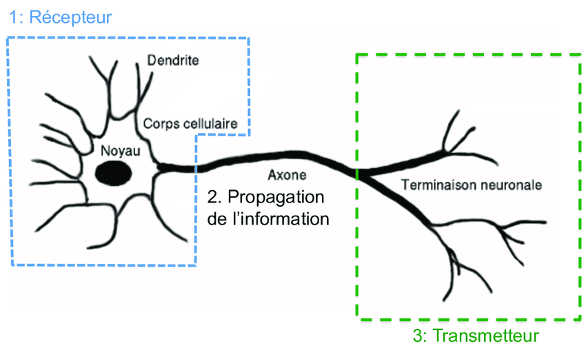
When building an artificial neural network or deep learning algorithm, the basic building block is the neuron. A neuron takes one or more inputs, which are simply numbers, performs some computation, and outputs another number. These outputs can then be used as inputs for other neurons. In this way, many neurons can be simulated at the same time to create a network.

In this diagram, three neurons are shown working together. They input a few numbers, perform computation, and output other numbers. However, it's important to note that while there is a loose analogy between biological neurons and artificial neurons, we currently have a limited understanding of how the human brain actually works.

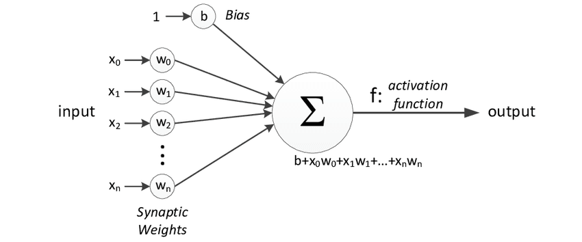
In summary, neural networks were created with the goal of mimicking the way the human brain learns and thinks. While the technology has come a long way since its inception, the original motivations remain an important part of how we think about neural networks today.

Demand Prediction

When building a neural network, it's important to understand the basic building block: the neuron. A neuron takes one or more inputs, which are simply numbers, performs some computation, and outputs another number. These outputs can then be used as inputs for other neurons. In this way, many neurons can be simulated at the same time to create a network.

To illustrate this concept, let's take an example of demand prediction for T-shirts.

• The goal is to predict if a T-shirt will be a top seller or not, based on data such as the price of the T-shirt and whether or not it became a top seller in the past.
• This type of application is used by retailers to plan better inventory levels and marketing campaigns.

In this example, the input feature x is the price of the T-shirt, and the goal is to predict if a particular T-shirt will be a top seller or not. To do this, we use logistic regression to fit a sigmoid function to the data. The output of the prediction is represented by the formula: f(x) = 1/1 + e^(-wx + b) where w and b are parameters learned during the training of the model.

This output, which we denote as a, represents the probability of the T-shirt being a top seller. Another way to think of it is that this logistic regression unit can be thought of as a simplified model of a single neuron in the brain. It takes in the input feature, price, and computes the output, probability of the T-shirt being a top seller.

To create a neural network, we take a number of these logistic regression units and wire them together to make a final prediction. In this example, we have 4 features to predict whether or not a T-shirt is a top seller. The features are:

• The price of the T-shirt
• The shipping costs
• The amounts of marketing of that particular T-shirt
• The material quality, is this a high-quality, thick cotton versus maybe a lower quality material?

Each of these features is input into a separate logistic regression unit, which compute the probability of T-shirt being affordable, having high awareness, or being perceived as high quality. These probabilities are then combined to make a final prediction of whether or not the T-shirt will be a top seller.

Each features is called, input layer as vector X (X->). They are inserted into hidden layer, called vector (A->) or activations, to go to the final output layer which provide the probability A.

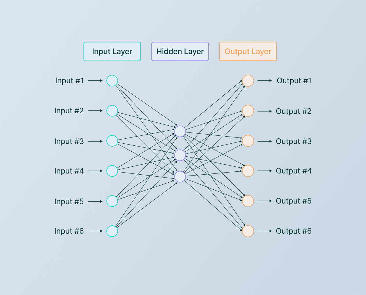
It's important to note that while the logistic regression algorithm is a simplified model of a single neuron in the brain, deep learning algorithms do work very well in practice. Building a neural network involves taking a number of these neurons and wiring them together to make a prediction.

Neuronal network model

The building blocks of most neural networks are layers of neurons. In this article, we will explore how to construct a layer of neurons and how to use these building blocks to create a larger neural network.

As an example, let's consider a demand prediction problem where we have four input features fed into a hidden layer with three neurons. These three neurons then send their output to an output layer with one neuron.

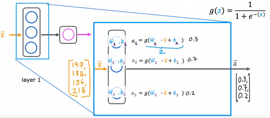
To understand how the hidden layer functions, let's take a closer look at the computations. The hidden layer inputs four numbers, which are then passed to each of the three neurons. Each neuron is essentially a logistic regression unit, with its own parameters (w and b). For example, the first neuron has parameters w_1 and b_1, and it outputs an activation value a, which is calculated as g(w_1 * x + b_1), where g is the logistic function and x is the input. This activation value, a_1, represents the probability of the input being highly affordable.

Similarly, the second neuron has parameters w_2 and b_2 and calculates an activation value a_2, which represents the probability of potential buyers being aware of the product. The third neuron has parameters w_3 and b_3 and calculates an activation value a_3. The vector of these three activation values, [a_1, a_2, a_3], is then passed to the final output layer of the neural network.

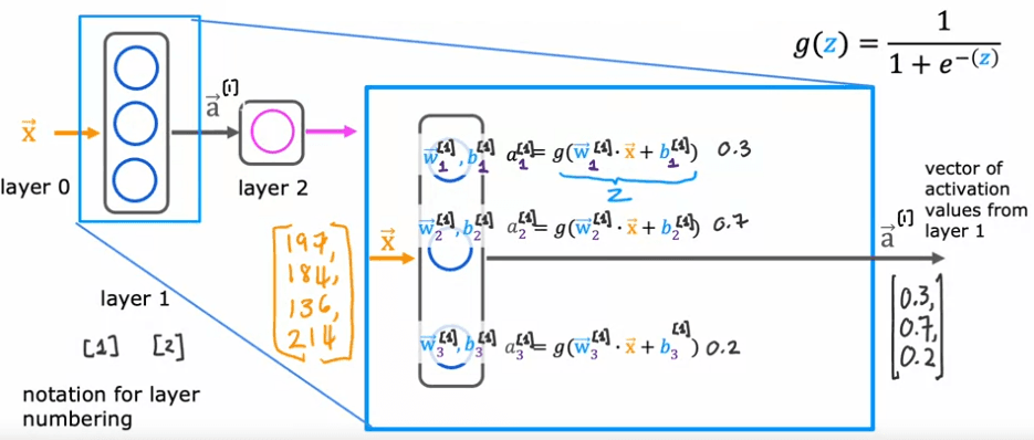
When building neural networks with multiple layers, it is useful to give the layers different numbers. By convention, the input layer is called layer 0, this hidden layer is called layer 1, and the output layer is called layer 2. However, today neural networks can have dozens or even hundreds of layers. To keep track of the different layers, we can use superscript square brackets to indicate which layer we are referring to. For example, a¹ refers to the output of layer 1, w²_1 refers to the parameters of the first unit in layer 1, and a³_1 refers to the activation value of the first neuron in layer 1.

In summary, a layer of neurons in a neural network is a fundamental building block, and by understanding how to construct a layer and how to use these building blocks, we can create large neural networks. Additionally, using notation such as superscript square brackets can help us keep track of different layers in a neural network.

More complex network

We will be exploring the concept of neural network layers and how they work to build more complex neural networks. A neural network is a system of algorithms that is designed to recognize patterns in data. It is made up of layers of interconnected nodes, each of which performs a specific function.

To better understand this concept, let's take a look at an example of a more complex neural network. This network has four layers, not counting the input layer, which is also called Layer 0. Layers 1, 2, and 3 are hidden layers, and Layer 4 is the output layer. By convention, when we say that a neural network has four layers, that includes all the hidden layers in the output layer, but we don't count the input layer.

Now, let's zoom in to Layer 3, which is the third and final hidden layer to look at the computations of that layer. Layer 3 inputs a vector, a_2, that was computed by the previous layer, and it outputs a_3, which is another vector. The computation that Layer 3 does to go from a_2 to a_3 is using three neurons or we call it three hidden units, then it has parameters w_1, b_1, w_2, b_2, and w_3, b_3 and it computes a_1 equals sigmoid of w_1. product with this input to the layer plus b_1, and it computes a_2 equals sigmoid of w_2. product with again a_2, the input to the layer plus b_2 and so on to get a_3. Then the output of this layer is a vector comprising a_1, a_2, and a_3.

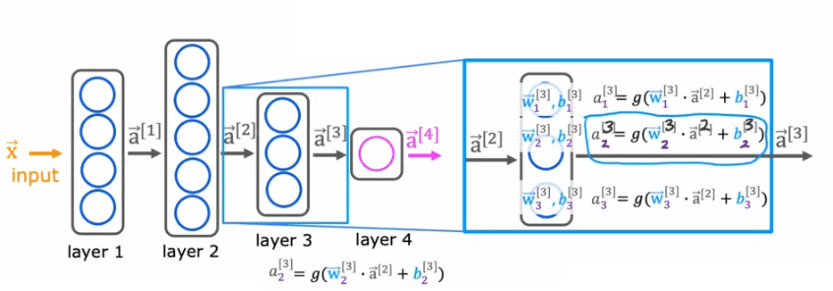
To apply the activation function, g, lets use the parameters of this same neuron. So w and b will have the same subscript 2 and superscript square bracket 3. The input features will be the output vector from the previous layer, which is layer 2. So that will be the vector 'a' superscript 2.

In summary, a neural network is a system of algorithms that is designed to recognize patterns in data. It is made up of layers of interconnected nodes, each of which performs a specific function. In this article, we used a more complex neural network example with four layers and zoomed in to Layer 3 to understand the computations that happen in each layer. We also discussed how the activation function and parameters are used to go from one layer to another. Understanding the concept of neural network layers and how they work is crucial in building more advanced neural networks.

Prediction - Forward propagation

The forward propagation algorithm is used to make inferences or predictions with a neural network. In this algorithm, input data is passed through the layers of the network, making computations at each layer, until the final output is produced.

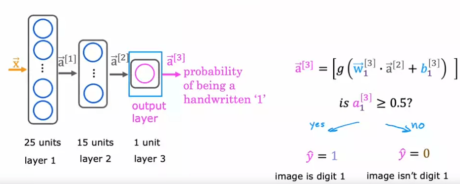
For example, in a binary classification problem of distinguishing between the handwritten digits zero and one, an eight by eight image is inputted into the network as 64 pixel intensity values. The neural network used in this example has two hidden layers, with the first hidden layer having 25 neurons and the second hidden layer having 15 neurons. The output layer produces the predicted probability of the image being the digit one versus zero.

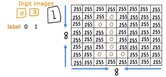
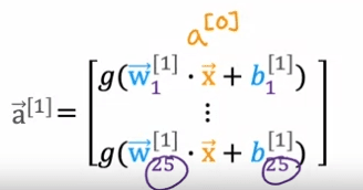
The first computation is to go from the input, X, to a1, which is done by the first layer of the first hidden layer using the formula on the right. The second step is to compute a2, which is done by the second hidden layer using a similar computation. The final step is to compute a3, which is done by the output layer using a similar computation. The output, a3, is also the output of the neural network and can be written as f(x).

We can define :

The sequence of computations made in the forward propagation algorithm is called forward propagation because the activations of the neurons are being propagated in the forward direction from left to right. This is in contrast to a different algorithm called backward propagation or backpropagation, which is used for learning. This type of neural network architecture, where the number of hidden units decreases as you get closer to the output layer, is a typical choice when choosing neural network architectures. With this understanding of forward propagation, you can now make inferences with your neural network.

Implementation with tensorflow

Roasting coffee beans at home can be a fun and rewarding experience, especially when using the right techniques and tools to achieve the perfect roast. One such tool is using a learning algorithm to optimize the quality of the beans during the roasting process. The temperature and duration of the roast are the inputs to the algorithm, and the output is the quality of the roasted coffee beans.

Using a dataset of different temperatures and durations, as well as labels indicating the quality of the roasted coffee beans, a supervised learning algorithm such as a regression algorithm can be trained to predict the quality of the roast based on the temperature and duration inputs. This can help ensure that the coffee beans are roasted to perfection every time.

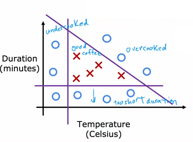
In a simplified example, the dataset shows that if the beans are cooked at too low of a temperature, they will be undercooked. If they are not cooked for long enough, they will also be undercooked. And if they are cooked for too long or at too high of a temperature, they will be burnt. Only points within a specific temperature and duration range will result in good coffee.

This example is simplified, but in actuality, there have been serious projects using machine learning to optimize coffee roasting. Using a neural network, the temperature and duration inputs are passed through layers of the network, making computations at each layer, until the final output is produced, which is the predicted quality of the roast.

In this example, a dense layer with 3 units and a sigmoid activation function is used for the first hidden layer and a dense layer with 1 unit and a sigmoid activation function is used for the second hidden layer. The final output, a2, is then thresholded at 0.5 to produce a binary classification of good or bad coffee. The additional details such as how to load the TensorFlow library and the parameters of the neural network can be found in the lab.

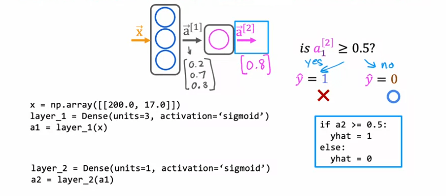
This is an example of forward propagation, which is the sequence of computations made in the neural network to go from the input to the final output. It's called forward propagation because the activations of the neurons are being propagated in the forward direction from left to right. This is in contrast to a different algorithm called backward propagation or backpropagation, which is used for learning.

Tensorflow explications

In this sections, we will be discussing how to build a neural network in TensorFlow. By now, you should have a good understanding of how to build layers and perform forward propagation in TensorFlow. We will be taking all of that knowledge and putting it together to create a complete neural network.

One way to build a neural network in TensorFlow is to manually initialize the data, create layer one, compute the activations, create layer two, and compute the activations again. This method can be time-consuming and tedious. However, TensorFlow has a simpler way of building a neural network called the sequential function.

The sequential function allows us to tell TensorFlow to take two layers and string them together to form a neural network. This eliminates the need for manual computation and allows TensorFlow to do a lot of the work for us. For example, let's say we have a training set like this:

 X = np.array([[1,2], [3,4], [5,6], [7,8]])
Y = np.array([0, 1, 1, 0])

Given the data, X and Y, we can train the neural network by calling the following two functions:

 model.compile(...)
model.fit(X, Y)

We will learn more about these functions next week, but for now, just know that they tell TensorFlow to take the neural network we created with the sequential function and train it on the data, X and Y.

In order to perform inference on a new example, we simply call the model.predict() function on a new input, X_new. This will output the corresponding value of the final layer, without the need for manual computation.

In addition to this, TensorFlow also has a convention of not explicitly assigning the layers to variables, but instead using the following code:

 model = Sequential()
model.add(Dense(3, activation='sigmoid'))
model.add(Dense(1, activation='sigmoid'))

This way of coding is more commonly seen in TensorFlow code, and it's the same as the previous example, but simpler.

In summary, building a neural network in TensorFlow is made easy with the use of the sequential function. It allows for faster and more efficient training and inference, and the convention of not explicitly assigning layers to variables also simplifies the code. Next week, we will delve deeper into the specific parameters used in the model.compile() and model.fit() functions, as well as other tips and tricks for coding in TensorFlow.

Numpy

we will be discussing how to implement forward propagation from scratch in Python. This is not only useful for gaining intuition about what's happening in libraries like TensorFlow and PyTorch, but also for those who may want to build something even better than these frameworks in the future.

We will be using a coffee roasting model as an example to demonstrate the process of forward propagation. The first step is to import the necessary libraries:

 import numpy as np

The parameters and biases are initialized as follows:

 w1_1, w1_2, w1_3 = 1.2, -3, 4
b1_1, b1_2, b1_3 = -1, 2, -0.5
w2_1 = -1
b2_1 = 0.5

The input feature vector is also initialized:

 x = np.array([1, 2])

The first value to compute is a1_1, which is the first activation value of a1. To compute this, we have parameters w1_1 and b1_1. We compute z1_1 as the dot product between the parameter w1_1 and the input x, and add b1_1. Finally, a1_1 is equal to the sigmoid function applied to z1_1:

 z1_1 = np.dot(w1_1, x) + b1_1
a1_1 = 1 / (1 + np.exp(-z1_1))

We repeat the process to compute a1_2 and a1_3 using the corresponding parameters and biases:

 z1_2 = np.dot(w1_2, x) + b1_2
a1_2 = 1 / (1 + np.exp(-z1_2))
z1_3 = np.dot(w1_3, x) + b1_3
a1_3 = 1 / (1 + np.exp(-z1_3))

We then group these values together into an array to give the output of the first layer, a1:

 a1 = np.array([a1_1, a1_2, a1_3])

We then implement the second layer. The output a2 is computed using the dot product of a1 and the parameter w2_1, added to the bias term b2_1, and applying the sigmoid function:

 z2_1 = np.dot(w2_1, a1) + b2_1
a2_1 = 1 / (1 + np.exp(-z2_1))

And that's it, that's how you can implement forward propagation from scratch in Python using numpy. Of course, this is a very basic example and for a more general neural network, the process can be simplified using loops and functions. But this example provides a solid foundation for understanding the underlying concepts and mechanics of forward propagation.

we will explore how to implement forward propagation from scratch in Python. This will help us gain a better understanding of what's happening behind the scenes in popular libraries like TensorFlow and PyTorch. It's important to note that this is not something that I would recommend for most people, as these libraries are powerful and efficient tools. However, understanding how to implement forward prop from scratch can be beneficial for anyone who wants to build something even better than TensorFlow and PyTorch.

Let's start by defining a function to implement a dense layer, which is a single layer of a neural network. We will call this function "dense". The dense function takes as input the activation from the previous layer, as well as the parameters w and b for the neurons in a given layer.

Here is an example of how the dense function can be used to implement forward prop in a single layer:

 import numpy as np

def sigmoid(z):
    return 1 / (1 + np.exp(-z))

def dense(a, w, b):
    units = w.shape[1]
    a = np.zeros(units)
    for j in range(units):
        w_j = w[:, j]
        z = np.dot(w_j, a) + b[j]
        a[j] = sigmoid(z)
    return a

x = np.array([1, 2, 3])
w1 = np.array([[1, 2, -1], [-3, 4, 1], [2, -1, 3]])
b1 = np.array([-1, 1, 2])
a1 = dense(x, w1, b1)
print(a1)

In this example, we have three neurons in the first layer and the parameters w1, w2, and w3 are stacked into a matrix. Similarly, the parameters b1, b2, and b3 are stacked into a 1D array. The dense function takes as input the activation from the previous layer, and the parameters for the current layer, and it returns the activations for the next layer.

Given the dense function, we can string together a few dense layers sequentially in order to implement forward prop in a neural network. For example, given the input features x, we can compute the activations a1 as a1 = dense(x, w1, b1) where w1 and b1 are the parameters of the first hidden layer. Then we can compute a2 as dense(a1, w2, b2) where w2 and b2 are the parameters of the second hidden layer. We can continue this process for as many layers as we need in the neural network.

It's important to note that this is a simplified example and in practice, there are many optimization techniques that are used to improve the efficiency and accuracy of neural networks. However, by understanding the basics of how forward prop can be implemented from scratch in Python, we can better understand the inner workings of popular deep learning libraries like TensorFlow and PyTorch.

Training data with tensorflow

Building a logistic regression model involves several steps, including specifying how to compute the output given the input feature x and the parameters w and b. The first step is to define the logistic regression function, which predicts f(x) as the sigmoid function applied to the dot product of w and x plus b :

The second step is to specify the loss function, which measures how well the logistic regression model is performing on a single training example (x, y). The cost function, which is an average of the loss function computed over the entire training set, is also defined in this step.

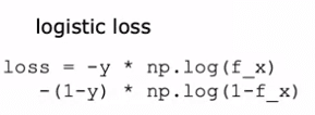
The final step is to use an algorithm, such as gradient descent, to minimize the cost function J(w, b) as a function of the parameters w and b. This is done by updating w and b using the derivative of J with respect to w and b, respectively. These three steps - specifying the output function, specifying the loss and cost functions, and minimizing the cost function - are the key steps in building and training a logistic regression model.

The same three steps can also be applied to training a neural network in TensorFlow. To specify the output function, the architecture of the neural network is defined, including the number of hidden units and the activation function used.

 model = Sequential(
    [
        tf.keras.Input(shape=(400,)),    #specify input size
        ### START CODE HERE ###
        Dense(25, activation='sigmoid', name = 'layer1'),
        Dense(15, activation='sigmoid', name = 'layer2'),
        Dense(1, activation='sigmoid', name = 'layer3')
        ### END CODE HERE ###
    ], name = "my_model"
)

The loss function, such as the binary cross entropy loss function, is specified in the second step:

 model.compile(

    loss=tf.keras.losses.BinaryCrossentropy(),

    optimizer=tf.keras.optimizers.Adam(0.001),

)

And the final step is to minimize the cost function using a function such as gradient descent:

 model.fit(
    X,y,
    epochs=20
)

Overall, the process of training a logistic regression model and a neural network in TensorFlow are similar and can be understood by breaking it down into these three steps.