Introduction

The most popular and widely used learning algorithm today is called binary classification, which is used to predict one of two possible outcomes, such as whether an email is spam or not, if a financial transaction is fraudulent or not, or if a tumor is malignant or benign. This type of classification problem is called binary classification because there are only two possible classes or categories.

The two classes or categories are often designated as no or yes, false or true, or zero or one. The negative class is often referred to as the false or zero class, and the positive class is often referred to as the true or one class.

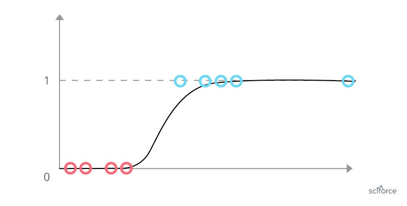
To build a classification algorithm, one approach is to use linear regression to fit a straight line to the data, but this method predicts all numbers between zero and one, rather than just the categories of zero and one. So a graph will be like :

Logistic regression

Introduction:

Logistic Regression is a commonly used classification algorithm that is used to predict binary outcomes. In this example, we will use it to classify whether a tumor is malignant or benign.

Problem:

We have a dataset where the horizontal axis is the size of the tumor and the vertical axis takes on only values of 0 and 1, because it is a classification problem. Linear regression is not a good algorithm for this problem.

Solution:

Logistic regression is used to fit an S-shaped curve to the dataset. For example, if a patient comes in with a tumor of a certain size, the algorithm will output a value between 0 and 1, suggesting the likelihood of the tumor being malignant or benign.

Sigmoid Function:

To build the logistic regression algorithm, we use an important mathematical function called the Sigmoid function, also referred to as the logistic function. The Sigmoid function outputs a value between 0 and 1, based on the input variable Z. The formula of g(z) is equal to 1 over 1 plus e to the negative z, where e is a mathematical constant that takes on a value of about 2.7.

We can represent the plot like this :

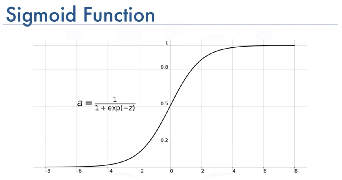
Note that we have positive and negative value for the horyzontal values (Z).

Building the Logistic Regression Model:

In the first step, we define a straight line function, like a linear regression function, which is represented by the variable Z. The next step is to take this value of Z and pass it through the Sigmoid function, which is represented by the variable g(z). This function outputs a value between 0 and 1. When z is large, g(z) is close to 1 and when z is a large negative number, g(z) is close to 0. When z is equal to 0, g(z) is equal to 0.5. This Sigmoid function is used to build the logistic regression model, which inputs a feature or set of features and outputs a number between 0 and 1

Output:

The logistic regression model takes in a set of features (i.e. input data) and outputs a value between 0 and 1, which can then be used to classify the input into one of the two possible classes. The next step is to interpret the output of the logistic regression model and make a decision based on the result.

We can define the formula as : 𝑓𝑤->,𝑏(𝑥->)=𝑤->*𝑥->+𝑏 where 𝑧 = 𝑤->*𝑥->+𝑏

We know that the sigmoide formula is : 𝑔(𝑧)=1/(1+𝑒−𝑧) We can by the way say : *𝑓𝑤->,𝑏(𝑥->) = 1/(1+𝑒−(𝑤->𝑥->+𝑏))

Example :

• X is "tumor size"
• Y is 0 (not malignant) or 1 (malignant)

𝑓𝑤->,𝑏(𝑥->) = 0.7 means that we have 70% of chance that the tumor is malignant

Implementation

Let's import our dependencies :

import numpy as np
import matplotlib.pyplot as plt
from plt_one_addpt_onclick import plt_one_addpt_onclick
from lab_utils_common import draw_vthresh

We can add our value and use the exponential function to calculate them :

# Create an input array and use the exp function to calculate the exponential of each element
input_array = np.array([1,2,3])
exp_array = np.exp(input_array)

# Print the input and output of the exp function
print("Input to exp:", input_array)
print("Output of exp:", exp_array)

Result :

Input to exp: [1 2 3]
Output of exp: [ 2.72 7.39 20.09]
Input to exp: 1
Output of exp: 2.718281828459045

We can apply our sigmoid formula : 1/(1+np.exp(-z))

# Define the sigmoid function
def sigmoid(z):
"""
Compute the sigmoid of z

Args:
z (ndarray): A scalar, numpy array of any size.

Returns:
g (ndarray): sigmoid(z), with the same shape as z

"""
g = 1/(1+np.exp(-z))

return g

We can calculate our function and display it into a graph :

# Create an array of values for z
z_tmp = np.arange(-10,11)

# Calculate sigmoid(z) for each value in the z_tmp array
y = sigmoid(z_tmp)

# Print the input and output of the sigmoid function
np.set_printoptions(precision=3)
print("Input (z), Output (sigmoid(z))")
print(np.c_[z_tmp, y])

# Plot z vs sigmoid(z)
fig,ax = plt.subplots(1,1,figsize=(5,3))

plots(1,1,figsize=(5,3))
ax.plot(z_tmp, y, c="b")

#Add title, labels and vertical threshold line to the plot
ax.set_title("Sigmoid function")
ax.set_ylabel('sigmoid(z)')
ax.set_xlabel('z')
draw_vthresh(ax,0)

We have now an example :

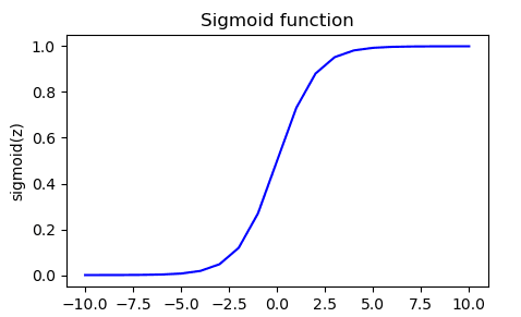
With values printed :

Input (z), Output (sigmoid(z))
[[-1.000e+01 4.540e-05]
[-9.000e+00 1.234e-04]
[-8.000e+00 3.354e-04]
[-7.000e+00 9.111e-04]
[-6.000e+00 2.473e-03]
[-5.000e+00 6.693e-03]
[-4.000e+00 1.799e-02]
[-3.000e+00 4.743e-02]
[-2.000e+00 1.192e-01]
[-1.000e+00 2.689e-01]
[ 0.000e+00 5.000e-01]
[ 1.000e+00 7.311e-01]
[ 2.000e+00 8.808e-01]
[ 3.000e+00 9.526e-01]
[ 4.000e+00 9.820e-01]
[ 5.000e+00 9.933e-01]
[ 6.000e+00 9.975e-01]
[ 7.000e+00 9.991e-01]
[ 8.000e+00 9.997e-01]
[ 9.000e+00 9.999e-01]
[ 1.000e+01 1.000e+00]]

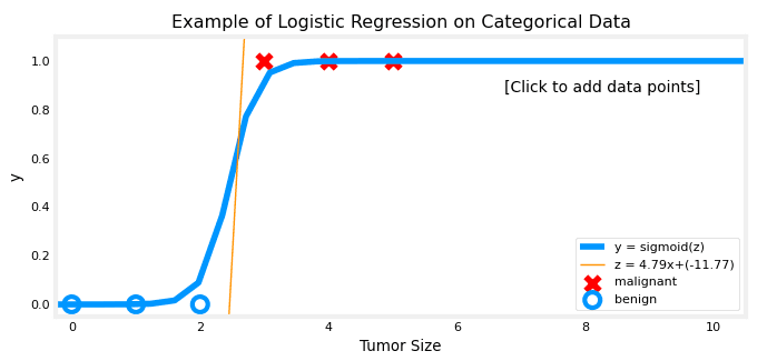
Now we can apply logistic regression to the categorical data :

#Create training data for x and y
x_train = np.array([0., 1, 2, 3, 4, 5])
y_train = np.array([0, 0, 0, 1, 1, 1])

#Initialize weight and bias
w_in = np.zeros((1))
b_in = 0

#Close all existing plots
plt.close('all')

#Plot the training data with the addpt function
addpt = plt_one_addpt_onclick(x_train,y_train, w_in, b_in, logistic=True)

We should have this graph displayed :

Decision boundary

In logistic regression, the goal is to predict whether the value of y is 0 or 1. To do this, a threshold is set, and if the predicted probability of y being 1 (calculated using the Sigmoid function) is greater than or equal to the threshold, the prediction is that y is 1.

Conversely, if the predicted probability is less than the threshold, the prediction is that y is 0. A common threshold value is 0.5, meaning that if f(x) (the output of the Sigmoid function) is greater than or equal to 0.5, y is predicted to be 1, and if f(x) is less than 0.5, y is predicted to be 0.

To visualize how the model makes predictions, an example is provided using a classification problem with two features: x1 and x2.

• The logistic regression model uses the function f(x) = g(z), where z = w1x1 + w2x2 + b.
• The line where wx + b = 0 is called the decision boundary and separates the points where the model predicts y to be 1 and y to be 0.
• This decision boundary is represented by a straight line.
• The decision boundary (Z= W->*X-> +b) depends on the values of the parameters w1, w2, (which are equals to 1) and b (-1). So let's say : Z= X(1,2) + X(2,2) -1 = 0 Where (Z= 3), which predict ^y = 1.

However, in more complex examples, the decision boundary may not be a straight line. For example, by using polynomial features, z can be set to be w1x1^2 + w2x2^2 + b, in this case, the decision boundary will be a curved line. We can say :

We know that the sigmoide formula is : 𝑓𝑤->,𝑏(𝑥->) = 𝑔(𝑤1𝑥1+𝑤2𝑥2+𝑏)

The decision boundary can also be non-linear. For example, the decision boundary could be a curve or even an oval, among other possible shapes.

Cost function

The cost function in logistic regression is used to measure how well a specific set of parameters fits the training data. This helps us to choose better parameters for our model.

Example: we have a training set for our logistic regression model, where each row corresponds to a patient visiting the doctor and being diagnosed with a condition. The training set has

• m number of examples
• Each with n features such as tumor size and patient age.

Size of tumor	Age	Malignant
24	30	1
10	32	0
5	23	0
5	12	1

Based of what we said :

• M is the number of training, m = 3
• Each training, i has n data, here n = 2
• The target label Y can take on only two values, 0 or 1

The logistic regression model is defined by the equation: f(x) = 1/(1+e^(-wx-b))

How can we choose parameter W and B ?

The squared error cost function is not an ideal choice for logistic regression because when the cost function is plotted using this value of f(x), it becomes a non-convex cost function with multiple local minima. Gradient descent can get stuck in these local minima, instead of converging to the global minimum. Let reproduce by a graph :

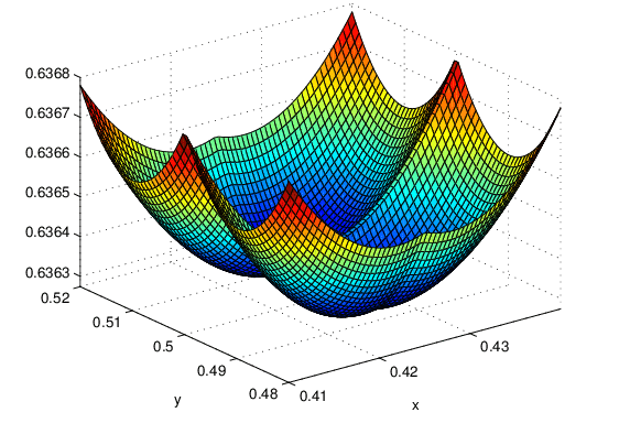
To overcome this, a different cost function is used for logistic regression, one that makes the cost function convex again.

The new cost function is defined as : J(w,b) = 1/n * ∑L(f(x),y)

Where L is the loss on a single training example and is a function of the prediction of the learning algorithm, f(x) and the true label y.

So : 𝑙𝑜𝑠𝑠(𝑓𝐰,𝑏(𝐱(𝑖)),𝑦(𝑖)) which is the cost for a single data point as :

• 𝑓𝐰,𝑏(𝐱(𝑖)) is the model's prediction, while 𝑦(𝑖) is the target value.
• 𝐰,𝑏(𝐱(𝑖))=𝑔(𝐰⋅𝐱(𝑖)+𝑏) where function 𝑔 is the sigmoid function.

The loss function used in logistic regression is characterized by its use of two distinct curves, one for when the target label is 0 (y=0) and another for when the target label is 1 (y=1). These curves work together to provide the desired behavior for a loss function, which is to be zero when the prediction matches the target and to rapidly increase in value as the prediction differs from the target. As seen in the graph, the loss function is zero when the prediction matches the target, and it increases as the prediction differs from the target.

This loss function can be visualized as a graph and provides insight into how well the model is performing on a single training example. By summing up the losses on all the training examples, we can ensure that the overall cost function is convex and gradient descent can converge to the global minimum.

We can simply this cost function to be more easy to memorize :

𝐽(𝐰,𝑏)=1𝑚∑𝑖=0𝑚−1[𝑙𝑜𝑠𝑠(𝑓𝐰,𝑏(𝐱(𝑖)),𝑦(𝑖))]

where

𝑙𝑜𝑠𝑠(𝑓𝐰,𝑏(𝐱(𝑖)),𝑦(𝑖)) is the cost for a single data point, which is: 𝑙𝑜𝑠𝑠(𝑓𝐰,𝑏(𝐱(𝑖)),𝑦(𝑖))=−𝑦(𝑖)log(𝑓𝐰,𝑏(𝐱(𝑖)))−(1−𝑦(𝑖))log(1−𝑓𝐰,𝑏(𝐱(𝑖)))

where m is the number of training examples in the data set and :

Implementation

import numpy as np
import matplotlib.pyplot as plt
from lab_utils_common import plot_data, sigmoid, dlc

we can define our dataset as :

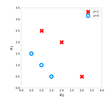
X_train = np.array([[0.5, 1.5], [1,1], [1.5, 0.5], [3, 0.5], [2, 2], [1, 2.5]]) #(m,n)
y_train = np.array([0, 0, 0, 1, 1, 1]) 

Let's draw this data using cross and round :

fig,ax = plt.subplots(1,1,figsize=(4,4))
plot_data(X_train, y_train, ax)

# Set both axes to be from 0-4
ax.axis([0, 4, 0, 3.5])
ax.set_ylabel('$x_1$', fontsize=12)
ax.set_xlabel('$x_0$', fontsize=12)
plt.show()

Plot should display :

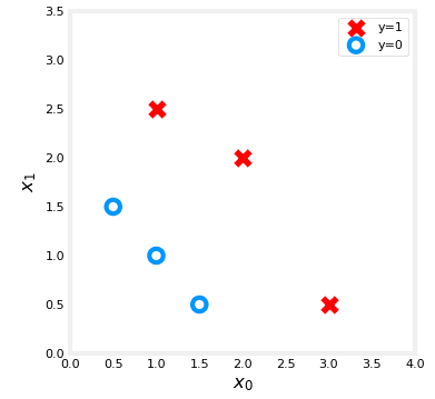
We can create our function previously define as :

def compute_cost_logistic(X, y, w, b):
"""
Computes cost

Args:
X (ndarray (m,n)): Data, m examples with n features
y (ndarray (m,)) : target values
w (ndarray (n,)) : model parameters
b (scalar) : model parameter

Returns:
cost (scalar): cost
"""

m = X.shape[0]
cost = 0.0
for i in range(m):
z_i = np.dot(X[i],w) + b
f_wb_i = sigmoid(z_i)
cost += -y[i]*np.log(f_wb_i) - (1-y[i])*np.log(1-f_wb_i)

cost = cost / m
return cost

We can now apply it and check the cost :

w_tmp = np.array([1,1])
b_tmp = -3
print(compute_cost_logistic(X_train, y_train, w_tmp, b_tmp))

result should be : 0.36686678640551745

Now, let's see what the cost function output is for a different value of 𝑤 .

In a previous lab, you plotted the decision boundary for 𝑏=−3,𝑤0=1,𝑤1=1 . That is, you had b = -3, w = np.array([1,1]).

Let's say you want to see if 𝑏=−4,𝑤0=1,𝑤1=1 , or b = -4, w = np.array([1,1]) provides a better model.

Let's first plot the decision boundary for these two different 𝑏 values to see which one fits the data better.

For 𝑏=−3,𝑤0=1,𝑤1=1 , we'll plot −3+𝑥0+𝑥1=0 (shown in blue) For 𝑏=−4,𝑤0=1,𝑤1=1 , we'll plot −4+𝑥0+𝑥1=0 (shown in magenta)

Gradient Descent

The goal of logistic regression is to find the values of the parameters w and b that minimize the cost function J of w and b.

The method used to achieve this goal is gradient descent. The cost function J is defined as the average of the error term, which is the difference between the predicted label y and the actual label y.

To minimize J, the derivative of J with respect to w and b is calculated using calculus. The derivative with respect to w is 1/m times the sum of the error term multiplied by the j feature of the training example i.

The derivative with respect to b is similar, but without the multiplication by x_j. These derivatives are plugged into the gradient descent algorithm, and the parameters are updated simultaneously.

Logistic regression is different from linear regression because the function f of x is defined as the sigmoid function applied to wx plus b, rather than just wx plus b. Gradient descent can also be monitored to ensure convergence, and feature scaling can be used to speed up the process. Vectorization can also be used to make gradient descent run faster for logistic regression.

Based on what we say we can isolate this formula :

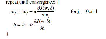
This 2 equations looks like exactly the same than for linear. Do not forget something, the definition for the function F(x) has changed, by using sigmoid !

Where each iteration performs simultaneous updates on 𝑤𝑗 for all 𝑗 , where

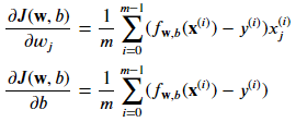
The parameters :

• m is the number of training examples in the data set
• 𝑓𝐰,𝑏(𝑥(𝑖)) is the model's prediction, while 𝑦(𝑖) is the target

The Gradient Descent algorithm implementation has two main components:

The loop implementing the gradient descent equation (1). This is typically referred to as the "gradient_descent" function and is usually provided in optional and practice labs. The calculation of the current gradient, as per equations (2,3) above. This is typically referred to as the "compute_gradient_logistic" function and is usually the part of the implementation that students are asked to complete in practice labs. The "compute_gradient_logistic" function is responsible for calculating the gradient for all 𝑤𝑗 and 𝑏 and is described as follows:

Initialize variables to accumulate the gradients dj_dw and dj_db For each example in the dataset: a. Calculate the error for that example 𝑔(𝐰⋅𝐱(𝑖)+𝑏)−𝐲(𝑖) b. For each input value 𝑥(𝑖)𝑗 in that example, multiply the error by the input 𝑥(𝑖)𝑗 and add it to the corresponding element of dj_dw (equation 2 above) c. Add the error to dj_db (equation 3 above) Divide dj_db and dj_dw by the total number of examples (m) Note that 𝐱(𝑖) in numpy is represented as X[i,:] or X[i] and 𝑥(𝑖)𝑗 is X[i,j]

We can implement this, first let import our dependencies :

import copy, math
import numpy as np
import matplotlib.pyplot as plt
from lab_utils_common import dlc, plot_data, plt_tumor_data, sigmoid, compute_cost_logistic
from plt_quad_logistic import plt_quad_logistic, plt_prob

Let's load some training dataset :

# Load the training dataset
X_train = np.array([[0.5, 1.5], [1,1], [1.5, 0.5], [3, 0.5], [2, 2], [1, 2.5]])
y_train = np.array([0, 0, 0, 1, 1, 1])

We will plot this data using our helper (can be find on git) :

fig,ax = plt.subplots(1,1,figsize=(4,4))
plot_data(X_train, y_train, ax)

# Set the plot limits and labels
ax.axis([0, 4, 0, 3.5])
ax.set_ylabel('$x_1$', fontsize=12)
ax.set_xlabel('$x_0$', fontsize=12)
plt.show()

Fine we should have this result :

Now let's create our function based on our formula :

def compute_gradient_logistic(X, y, w, b):
"""
Computes the gradient of the logistic cost function with respect to the parameters w and b.
"""
m,n = X.shape
dj_dw = np.zeros((n,)) #(n,)
dj_db = 0.

for i in range(m):
f_wb_i = sigmoid(np.dot(X[i],w) + b) #(n,)(n,)=scalar
err_i = f_wb_i - y[i] #scalar
for j in range(n):
dj_dw[j] = dj_dw[j] + err_i * X[i,j] #scalar
dj_db = dj_db + err_i
dj_dw = dj_dw/m #(n,)
dj_db = dj_db/m #scalar

return dj_db, dj_dw

Let compute, and return some result to have a view of our algorithm :

X_tmp = np.array([[0.5, 1.5], [1,1], [1.5, 0.5], [3, 0.5], [2, 2], [1, 2.5]])
y_tmp = np.array([0, 0, 0, 1, 1, 1])
w_tmp = np.array([2.,3.])
b_tmp = 1.
dj_db_tmp, dj_dw_tmp = compute_gradient_logistic(X_tmp, y_tmp, w_tmp, b_tmp)
print(f"dj_db: {dj_db_tmp}" )
print(f"dj_dw: {dj_dw_tmp.tolist()}" ) 

The code below implements the equation (1) above. It is important to take a moment to locate and compare the functions used in the routine with the equations mentioned above.

def gradient_descent(X, y, w_in, b_in, alpha, num_iters):
J_history = []
w = copy.deepcopy(w_in)
b = b_in

for i in range(num_iters):
# Compute the gradient and update the parameters
dj_db, dj_dw = compute_gradient_logistic(X, y, w, b)

w = w - alpha * dj_dw
b = b - alpha * dj_db

# Save the cost function value at each iteration
if i<100000:
J_history.append( compute_cost_logistic(X, y, w, b) )
# Print the cost function value every 10th iteration or if less than 10 iterations
if i% math.ceil(num_iters / 10) == 0:
print(f"Iteration {i:4d}: Cost {J_history[-1]} ")
# Return the final updated parameters and the cost function history for plotting 
return w, b, J_history 

Run the gradient :

# Test the gradient computation function with a sample dataset and parameters
w_tmp = np.zeros_like(X_train[0])
b_tmp = 0.
alph = 0.1
iters = 10000

w_out, b_out, _ = gradient_descent(X_train, y_train, w_tmp, b_tmp, alph, iters)
print(f"\nupdated parameters: w:{w_out}, b:{b_out}")

Result :

Iteration 0: Cost 0.684610468560574
Iteration 1000: Cost 0.1590977666870456
Iteration 2000: Cost 0.08460064176930081
Iteration 3000: Cost 0.05705327279402531
Iteration 4000: Cost 0.042907594216820076
Iteration 5000: Cost 0.034338477298845684
Iteration 6000: Cost 0.028603798022120097
Iteration 7000: Cost 0.024501569608793
Iteration 8000: Cost 0.02142370332569295
Iteration 9000: Cost 0.019030137124109114

updated parameters: w:[5.28 5.08], b:-14.222409982019837

We can finally plot the result :

# Create a figure with specified size
fig,ax = plt.subplots(1,1,figsize=(5,4))
# Plot the probability of the logistic regression model with updated parameters
plt_prob(ax, w_out, b_out)

# Set labels for x and y axis
ax.set_ylabel(r'$x_1$')
ax.set_xlabel(r'$x_0$')
# Set axis limits
ax.axis([0, 4, 0, 3.5])
# Plot the original data points
plot_data(X_train,y_train,ax)

# Calculate the decision boundary
x0 = -b_out/w_out[0]
x1 = -b_out/w_out[1]
# Plot the decision boundary on the same plot
ax.plot([0,x0],[x1,0], c=dlc["dlblue"], lw=1)
# Show the plot
plt.show()

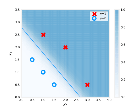
The plot above illustrates the probability of y=1, represented by the shading. The decision boundary is represented by the line at which the probability of y=1 is equal to 0.5. It separates the area where the probability of y=1 is greater than 0.5 from the area where it is less than 0.5. In other words, it is the line that separates the area where the model predicts y=1 from the area where it predicts y=0.