Introduction

Machine learning, invented in the 1960s, is a combination of two words: "machine," referring to a computer, robot, or any other device, while "learning" refers to the activity of discovering patterns in events where humans excel. It allows machines to acquire human knowledge without the limitations of human constraints such as strikes, fatigue, or illness. However, it is important to note that machine learning is not simply automation. Contrary to popular myth, machine learning is not the same as automation because it involves instructive and repetitive tasks without reflection beyond. If it were possible to hire many software programmers and continue to program new rules or extend old ones, the solution would become expensive over time due to the many variations that could arise.

Traditional Programming	Machine Learning
The computer applies a predefined set of rules to process input data and generate a result accordingly.	The computer attempts to emulate the human thought process by interacting with input data, the environment, and expected outcomes, from which it deduces patterns represented by one or more mathematical models. These models are then used to interact with future input data and produce results without explicit and directive instruction.

The field of machine learning is closely related to disciplines such as linear algebra, probability theory, statistics, and mathematical optimization. We often build machine learning models using statistical, probabilistic, and linear algebraic concepts and then optimize these models through mathematical optimization techniques.

Types of Learning

The primary function of machine learning is to explore and develop algorithms that can learn from historical data and make predictions on new input data. For a data-driven solution, it is necessary to define an evaluation function called a loss or cost function, which measures the effectiveness of the learning models.

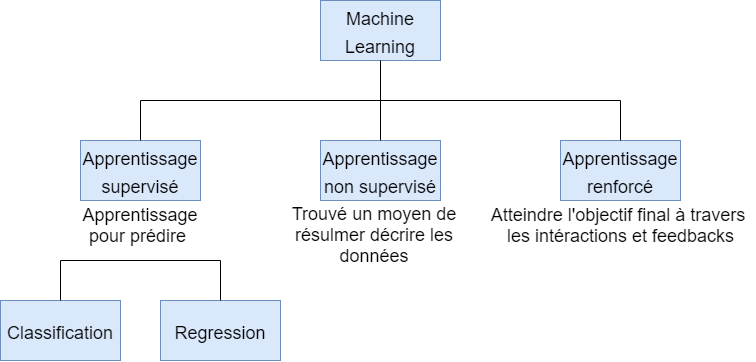
There are three categories of learning:

• Unsupervised learning: in which data does not have a pre-existing description, thus requiring identification of the structure of the data. Unlabeled data can be used to detect anomalies, such as fraud or faulty equipment, or to cluster customers with similar online behaviors for a marketing campaign.

• Supervised learning: in which data is provided with descriptions, objectives, and desired outcomes. Labeled data is then used to learn a rule that can be used to label new data with an unknown output. Labels are typically provided by event recording systems or evaluated by human experts. Supervised learning is used for facial and speech recognition, product or movie recommendations, sales forecasting, and spam detection.

• Reinforcement learning: which is used for applications such as industrial robotics, autonomous cars, and games such as AlphaGo. The main difference between reinforcement learning and supervised learning lies in interaction with the environment.

Here is the same text formatted as a code snippet:

vbnet Copy code

Types of Learning

Unsupervised learning can take two distinct forms:

• Unsupervised regression: which allows the prediction of continuous values such as housing prices, for example.
• Unsupervised classification: which allows finding the appropriate class label, for example, by analyzing positive/negative sentiment and predicting default payment.

In some cases, some training samples may be labeled while others are not. This leads to what is called semi-supervised learning.

Data

The current world produces an enormous amount of data, including both quality data and erroneous data. One of the main challenges in processing this data is its diversity and imprecision. Computers operate using electrical signals which are then translated into binary codes 0 and 1. In the field of programming language Python, for example, data is normally represented as numbers, images, or texts. However, for machine learning algorithms, it is often necessary to convert images and text into numerical data in order to process them effectively.

In the field of machine learning, data is often divided into three sets:

• Training sets
• Validation sets
• Test sets

Training sets are used to train learning models, while validation sets are used to evaluate the performance of these models during the learning process. Test sets are ultimately used to measure the performance of learning models on unknown data, and thus determine their actual effectiveness. To generalize learning models and make them applicable to unknown data, it is therefore crucial to use diverse and quality datasets, while taking into account the inaccuracies and differences that may exist between different types of data.

Overfitting, Underfitting, and Bias-Variance Tradeoff

Overfitting

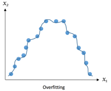
Overfitting, also known as overtraining, occurs when the learning model is too complex and is trained on too small a data set, resulting in excessive matching with existing observations. Although the model may work perfectly with training data, it may not be able to generalize and predict new observations outside of this data set.

Overfitting is often caused by an overuse of training data, which can lead to memorization rather than understanding of the model. This can be avoided using techniques such as cross-validation and hyperparameter tuning, which allow the selection of the most appropriate model and avoid biases.

Bias, on the other hand, is a measure of the average accuracy of a model's predictions compared to actual values. A model with high bias may be biased due to incorrect assumptions or the use of a model that is too simple to capture the complexity of the data. In the field of machine learning, it is important to find the right balance between bias and variance in order to maximize the predictive performance of the model.

note: ^y => prediction

High variance in a learning model means that it performs poorly on data sets that have not been seen before. Variance measures the model's ability to adapt to new assumptions, and therefore the variability of predictions. A model with high variance may be too complex and may overfit the training data, leading to poor performance on test data.

We can represent overfitting like this:

Prompt

Overfitting is often caused by excessive use of training data and overly complex models. By attempting to describe the learning rules based on too many parameters compared to the small number of observations, the model can overfit to the training data instead of capturing the underlying relationship. For example, if we have only a few training examples to distinguish between potatoes and tomatoes, and we try to deduce many features to distinguish them, our model may overfit the specific training examples rather than capturing the distinctive traits of potatoes and tomatoes.

Overfitting can also be caused by a model that is too complex and can excessively fit to the training data, which can lead to poor performance on the test data. For example, if we create a model that memorizes all the answers to all the questions in the training set, it may be very accurate on the training set, but it will be unable to generalize to new question examples.

Underfitting

Underfitting is a phenomenon that occurs when the model is unable to capture the trend or underlying structure of the data. This can occur if the model is too simple and does not contain enough parameters to capture the complexity of the data, or if the model is poorly chosen for the type of data in question.

Underfitting can also occur if we do not have enough data to adequately train the model. In this case, the model may be too generalized and not be able to capture subtle variations in the data.

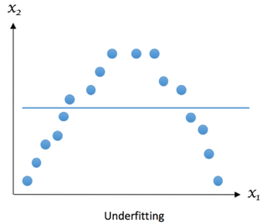
The desired outcome can be represented as follows:

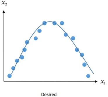
High bias is often associated with underfitting, as the model is unable to capture the underlying structure of the data. This can result in consistent but insufficient performance on both training and test sets, indicating low variance. To resolve underfitting, it is often necessary to use more complex models or add additional features to capture missing details in the data. Additionally, increasing the size of the dataset can also help improve the model performance and avoid underfitting.

Bias-Variance Tradeoff

We must avoid cases where either bias or variance becomes high. Does this mean we should always minimize both bias and variance? The answer is yes, if possible. However, in practice, there is an explicit tradeoff between the two, where decreasing one increases the other: this is the bias-variance tradeoff.

We want to create a model that can predict the election of a president. To do this, we conduct telephone surveys by zip code to obtain samples. We take random samples from one zip code and estimate that President X will be elected with a probability of 61%. However, President X is not elected, so why? The first thing we think of is the small size of the samples from only one zip code, which is also a source of high bias. People in a geographical area tend to share similar demographic data, leading to low variance in estimates. Can using samples from multiple zip codes correct this? Yes, but it could simultaneously lead to an increase in variance of the estimates: this is the bias-variance tradeoff.

We can measure mean squared error (MSE): given a set of training samples x1, x2, …, xn and their targets y1, y2, …, yn, we want to find a regression function (x) that correctly estimates the true relationship y(x).

Here, E represents the expectation or error. This error can be decomposed into bias and variance components following analytical derivation.

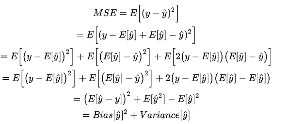
Bias measures the systematic error of estimates, while variance describes how much the estimation ŷ moves around its mean, E[y]. The more complex the learning model ŷ(x) is and the larger the size of the training samples, the more bias tends to decrease. However, this can also lead to an increase in the model's variance to better fit the additional data points.

Cross-Validation

The validation procedure is a crucial step in evaluating how models generalize to independent datasets in a given domain. In a conventional validation framework, the original data is usually partitioned into three subsets: 60% for training, 20% for validation, and 20% for testing. Although this is sufficient if we have enough training samples, otherwise, cross-validation is preferable.

In a cross-validation cycle, the original data is divided into two subsets: training and testing (or validation). Cross-validation is an efficient way to reduce variability and thus limit overfitting. There are mainly two cross-validation schemes used: the exhaustive scheme and the "k-fold" scheme.

The exhaustive scheme involves issuing a fixed number of observations at each turn as test samples, while using the remaining observations as training samples. This process is then repeated until all the different subsets of samples are used for testing at least once. Leave-One-Out-Cross-Validation (LOOCV) is an example of this scheme: for a dataset of size n, LOOCV requires n cycles of cross-validation. However, this can be slow when n becomes large.

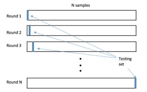
The "k-fold" scheme involves dividing the data into k equal subsets. Each subset is used in turn as a test set, while the other subsets are used as training sets. This process is repeated k times, using each subset once as a test set. The "k-fold" cross-validation is generally faster than the exhaustive scheme while producing more stable performance estimates.

Round
1	Test	Training	Training	Training	Training
2	Training	Test	Training	Training	Training
3	Training	Training	Test	Training	Training
4	Training	Training	Training	Test	Training
5	Training	Training	Training	Training	Test

"k-fold" cross-validation is generally preferable to Leave-One-Out-Cross-Validation (LOOCV) due to its lower variance. This is because "k-fold" cross-validation uses a block of samples for validation instead of one, as is the case with LOOCV.

However, nested cross-validation is a combination of cross-validations that has two distinct phases. The first phase, called internal cross-validation, is used to find the best model fit. It can be implemented in the form of "k-fold" cross-validation. In this phase, the model is fit on subsets of training samples and evaluated on subsets of validation samples.

The second phase, called external cross-validation, is used for evaluating the performance and statistical analysis of the model adjusted in the previous phase. This phase also uses a "k-fold" cross-validation, where the model is trained on subsets of the data and evaluated on test subsets different from those used in the internal phase.

By using nested cross-validation, we can evaluate the generalization ability of a model more accurately and robustly. This is particularly important when the dataset size is small or when we use complex models that can overfit the data.

Regularization

Regularization is a technique that involves adding parameters to the error function in order to limit the complexity of models. Polynomial models are more complex than linear models because the latter are determined by only two parameters: the intercept and the slope. The dimension of the coefficient search space for a line is therefore two. In contrast, a quadratic polynomial adds an additional coefficient for the quadratic term, which extends the search space to three dimensions. As a result, it is easier to find a high-order polynomial model that fits perfectly to the training data, and therefore more prone to overfitting, because its search space is larger than that of a linear model.

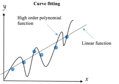
If a data scientist wants to equip their robot dog with the ability to identify strangers using their knowledge, they can use several machine learning methods. They can start by training a linear model, as this type of model is often preferable in terms of generalization to new data points. To avoid the negative effects of high polynomial orders, they can use regularization techniques to reduce their influence by imposing penalties. This would discourage complexity and obtain a less precise but more robust rule learned from the training data.

Sex	Age	Height	With Glasses	Colors	Label
Female	Middle	Medium	Yes	Black	Stranger
Male	Young	Small	Yes	White	Friend
Male	Senior	Small	Yes	Black	Stranger
Female	Young	Medium	Yes	White	Friend
Male	Young	Small	Yes	Red	Friend

If the robot uses these rules to identify strangers, it could conclude that any middle-aged woman of average height without glasses and dressed in black is a stranger, as well as any senior man of small stature without glasses and dressed in black. The robot could also identify someone else as their friend. However, while these rules may perfectly fit the training data, they are too complicated to generalize well to new visitors. To avoid overfitting, it is recommended to limit the model complexity using regularization techniques and stopping the learning procedure prematurely. Regularization should be maintained at an optimal level to avoid underfitting or excessive deviation of the model from the truth.

Feature Selection and Dimensionality Reduction

Data is typically represented in the form of a matrix where each column represents a feature, also known as a variable, and each row represents an example that can be used for supervised learning training or testing. Thus, the dimensionality of data corresponds to the number of features. Text and image data typically have high dimensionality, while stock market data has relatively low dimensionality.

Feature selection is an important process for constructing a quality model. It involves selecting a subset of relevant features for training the model while removing redundant or irrelevant features. Feature selection involves binary decisions for including or excluding a feature. This can lead to a large number of possible feature sets, up to 2^x for x features.

To avoid this combinatorial explosion, more advanced feature selection algorithms have been developed to identify the most useful signals and thus reduce the dimensionality of data. These algorithms allow for more efficient selection of the most relevant feature sets.

Data Preprocessing and Feature Engineering

Cross-Industry Standard Process for Data Mining (CRISP-DM):

Support from domain experts is important for business understanding and data understanding, as they have in-depth domain knowledge and can contribute to defining the business problem as well as understanding the data.

Data preparation requires technical skills to create training and testing data sets, and a domain expert who only knows Microsoft Excel may not be sufficient for this phase.

Modeling involves formulating a model and fitting the data to it.

Evaluation is important to determine how well the model fits the data, which allows verifying whether the business problem has been satisfactorily solved.

Deployment involves setting up the system in a production environment, so that the model can be used to solve the business problem.

Preprocessing

Data cleaning is an essential step in the machine learning process. To clean the data, it is necessary to understand the data itself. To do this, it is possible to analyze and visualize the data, depending on their type.

In the case of a table of numbers, it is important to check for missing values, how values are distributed, and what type of features we have. Values can follow different types of distributions, such as normal, binomial, Poisson, or others. Features can be binary (yes or no, positive or negative, etc.), categorical (continent of residence, etc.), or ordinal (high, medium, low). Features can also be quantitative (temperature in degrees or price in dollars).

When missing values are detected, it is important to decide how to handle them. It is possible to ignore these missing values, but this can lead to errors in the results. It is also possible to impute missing values by using the arithmetic mean, median, or mode of the valid values of a certain feature.

Label encoding

For machine learning to work, it is imperative that the data be in numerical form. If we provide a string such as "Ivan", the program will not be able to process the data unless we use specialized software. To convert a string to a numerical value, we can:

Label	Encoded Label
Africa	1
Europe	2
South America	3
North America	4
Other	6

This method can cause problems in some cases, as the learning algorithm can infer an implicit order (unless an explicit order is expected, such as bad=0, ok=1, good=2, excellent=3). In the previous mapping table, the ordinal encoding shows a difference of 4 between Asia and North America, which is counterintuitive as it is difficult to quantify these values. To remedy this, one-hot encoding can be used. This method uses dummy variables to encode categorical features.

Dummy variables are binary variables, represented as bits, that take on values of either 0 or 1. For example, to encode continents, we would use dummy variables such as "is_asia", which would be true if the continent is Asia and false otherwise. The number of dummy variables needed is equal to the number of unique labels, minus one. We can automatically infer one of the labels from the dummy variables as they are mutually exclusive. If all dummy variables are false, the correct label will be the one for which there is no dummy variable.

Label	IsAfrica	Is_Asia	Is_Europe	Is_sam	Is_nam
Africa	1	0	0	0	0
Europe	0	1	0	0	0
South America	0	0	1	0	0
North America	0	0	0	1	0
Other	0	0	0	0	1

When we use one-hot encoding to encode categorical data, this produces a matrix with a large number of zeros (representing false values) and a small number of non-zero values (representing true values). This matrix is called a sparse matrix as most of its elements are zero.

Scaling

It is common for the values of different features to differ by orders of magnitude, which can sometimes mean that the highest values dominate the smaller values. In such cases, there are several strategies for normalizing the data:

• Normalization involves subtracting the mean of the feature and dividing by the standard deviation. If the feature values are normally distributed, the normalized feature will be centered around zero with a variance of one, forming a Gaussian distribution.

• If the feature values are not normally distributed, we can use the median and interquartile range (IQR) to normalize. The IQR is the difference between the first and third quartile (or the 25th and 75th percentile).

• Another common strategy is to scale the features to a range from zero to one. This method is often used to normalize the data so that it is comparable between features. We will cover this method in our future examples.

Feature engineering

The process of creating or improving features is often based on common sense, domain knowledge, or prior experience. However, there is no guarantee that creating new features will improve the results. There are several techniques for creating new features:

• Polynomial transformation: if two features have a polynomial relationship, such as a2 + ab + b2, each term can be considered a feature. The interaction, such as ab, can be a sum, difference, or ratio rather than a product, and the number of features and polynomial order is not limited. However, complex polynomial relationships can be difficult to calculate and can lead to overfitting.

• Power transformation: transformation functions can be used to adjust numerical features to a normal distribution. For example, logarithm is a common transformation for values that vary by orders of magnitude. Box-Cox transformation can be used to find the best power to transform the data to a distribution closer to normal.

• Binning: feature values can be grouped into several bins. For example, if we are only interested in whether it rained on a given day, we can binarize precipitation values to get a true value if the precipitation value is non-zero, and a false value otherwise.

Model combination

By using multiple models to produce predictions, we can improve overall performance by reducing individual errors of each model. However, it is important to find a balance between model complexity and their ability to improve results.

Voting and averaging are two simple methods for combining predictions from multiple models. They are often used when the models have similar performance, but can also be weighted to give more weight to more reliable models. However, it should be noted that this approach may not work if the models are very different or if one of them is much less reliable than the others.

Bagging is a more advanced technique that can reduce the risks of overfitting and improve prediction stability. It involves creating multiple training data sets by sampling the data with replacement, and training a model for each set. The results of different models are then combined to produce a final prediction. This technique can be particularly useful for models that tend to overfit the training data.

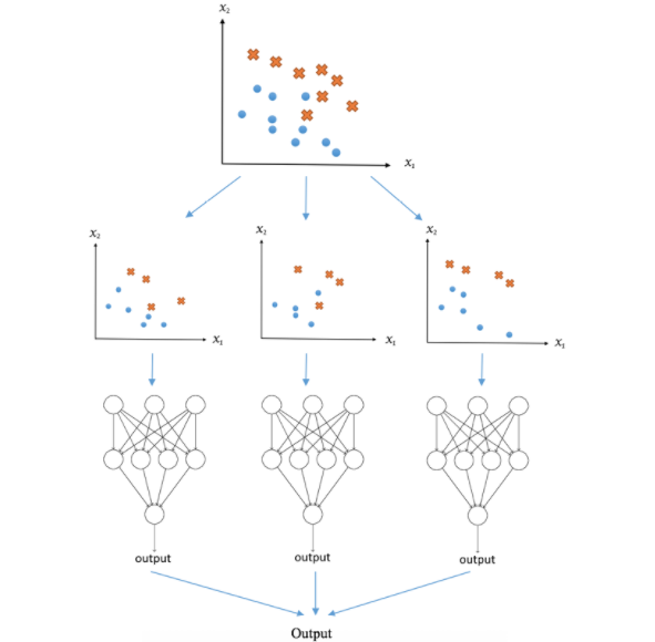
Ultimately, the choice of combination technique will depend on the characteristics of the model and data, as well as the specific goals of the project. It is important to consider multiple models and combination techniques to achieve the best possible results.