Description
Graphs are computational structures used in our everyday life:
- Cities that are interconnected
- Our social networks that connect us to each other
- Web pages
And many other cases that represent links between different actors. These graphs have allowed the development of algorithms aimed at solving complex problems.
Prerequisites Before we start, we will use one of the most popular languages in the world of machine learning: Python.
Here is the list of elements used in our exercise:
Jupyter==1.0.0 networkx==2.5 snap-stanford==5.0.0 matplotlib==3.2.2 pandas==1.1.3 scipy==1.6.2
Networkx will allow us to illustrate graph theory through various examples.
Simple undirected graph
An undirected graph (G) is defined by a set of vertices (V) and edges (E) or links connecting the vertices.
Thus, we can say that a graph is mathematically represented as: G = (V,E), where V is represented by a set of vertices V={ V1, .., Vn} that are connected by a set of edges that define the links between each vertex E= {{Vk, Vi} ... {Vi,Vn}}.
In the case of an undirected graph, the order of the defined edges does not matter, thus: {Vk, Vn} and {Vn, Vk} refer to the same edge (link).
So let's remember our first formulas:
- G = (V, E)
- V = { V1, .., Vn}
- E = {{Vk, Vi} ... {Vi,Vn}} where the set of links is not oriented
Graph theory also allows us to define:
- The order: number of vertices (V) in a graph.
- The size: number of edges (E) in a graph.
- The degree of a vertex: number of edges that are adjacent to it.
- The neighbors of a vertex: subset of vertices V' induced by all adjacent vertices
- The ego graph is a subgraph of G, composed of the vertices and edges adjacent to V.
Example
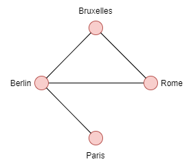
In the case of an undirected graph, the edges connecting Berlin to Paris {Berlin, Paris} are equal to {Paris, Berlin}; there is no distinction between these two edges.
- Order: 4 because we have 4 vertices (Berlin, Brussels, Paris, Rome)
- Degree of Brussels, Rome: 2
- Degree of Berlin: 3
- Degree of Paris: 1
Neighbors of each vertex:
- Paris={Berlin}
- Berlin={Bruxelles, Rome, Paris}
- Bruxelles={Rome, Berlin}
- Rome={Bruxelles, Berlin}
To illustrate this example, we need to create an undirected graph. To do this, nx.Graph() allows us to create this type of graph without specifying a direction. This method returns an object where all vertices and edges are accessible. Here are some useful methods:
| Function | Description | Return Type |
|---|---|---|
Graph() |
Returns an undirected graph | Graph |
Graph.number_of_edges() |
Returns the number of edges | int |
Graph.number_of_nodes() |
Returns the number of vertices | int |
Graph.degree() |
Returns an array representing the degree of each vertex | list |
Graph.neighbors() |
Returns an array representing the vertices and each of their neighbors | list |
Graph.ego_graph(Graph G, String nameOfGraph) |
Returns the neighbor subgraph | list |
Graph.add_nodes_from(V) |
Adds vertices | None |
Graph.add_edges_from(E) |
Adds edges | None |
Graph.remove_nodes_from(V) |
Removes vertices | None |
Graph.remove_edges_from(E) |
Removes edges | None |
Here's an example of creating an undirected graph and performing some useful methods:
import networkx as nx
G = nx.Graph()
V = {'Dublin', 'Paris', 'Milan', 'Rome'}
E = [('Milan','Dublin'), ('Milan','Paris'), ('Paris','Dublin'), ('Milan','Rome')]
G.add_nodes_from(V)
G.add_edges_from(E)
print(f"V = {G.nodes}")
print(f"E = {G.edges}")
print(f"Graph Order: {G.number_of_nodes()}")
print(f"Graph Size: {G.number_of_edges()}")
print(f"Degree for nodes: { {v: G.degree(v) for v in G.nodes} }")
print(f"Neighbors for nodes: { {v: list(G.neighbors(v)) for v in G.nodes} }")
Output:
V = ['Paris', 'Rome', 'Bruxelles', 'Berlin']
E = [('Paris', 'Berlin'), ('Rome', 'Berlin'), ('Rome', 'Bruxelles'), ('Bruxelles', 'Berlin')]
Graph Order: 4
Graph Size: 4
Degree for nodes: {'Berlin': 3, 'Paris': 1, 'Bruxelles': 2, 'Rome': 2}
Neighbors for nodes: {'Berlin': ['Rome', 'Paris', 'Bruxelles'], 'Paris': ['Berlin'], 'Bruxelles': ['Rome', 'Berlin'], 'Rome': ['Berlin', 'Bruxelles']}
We can also calculate an ego graph of a specific vertex for graph G:
ego_graph_berlin = nx.ego_graph(G, "Berlin")
print(f"Nodes: {ego_graph_berlin.nodes}")
print(f"Edges: {ego_graph_berlin.edges}")
Output:
Nodes: ['Paris', 'Milan', 'Dublin', 'Rome']
Edges: [('Paris', 'Milan'), ('Paris', 'Dublin'), ('Milan', 'Dublin'), ('Milan', 'Rome')]
## Graphe simple orienté (digraphs)
Un graphe orienté (**G**) est définit par un ensemble de Sommets (**V**) et d'arêtes (**E**) ou liens interconnectant les sommets.
Ainsi nous pouvons dire qu'un Graph est représenté mathématiquement comme : **G = (V,E)** où V est représenté par un ensemble de sommets **V={ V1, .., Vn}** qui sont connecté par un ensemble d'arêtes qui définit les liens entre chaque sommet **E= {{Vk, Vi} ... {Vi,Vn}}**.
Dans le cas d'un graphe orienté, l'ordre des arêtes défini a une importance, ainsi : **{Vk, Vn}** et **{Vn, Vk}** ne désigne pas la même arête. **{Vk, Vn}**: Cela signifie que Vk va vers Vn et que Vn pourrait ne pas aller vers Vk si on ne le stipule pas.
Ainsi nous étendons le degré à un type de dégré intérieur et extérieux :
* deg-(v): Pour un sommet V, c'est le nombre de têtes adjacents à v
* deg+(v): Pour un sommet V, c'est le nombre de queue adjacents à v
**Exemple** 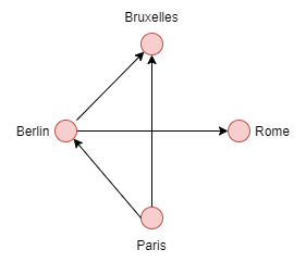
* deg-(v) de Bruxelles: 2
* deg+(v) de Bruxelles: 0
* deg-(v) de Paris: 0
* deg+(v) de Paris: 2
* deg-(v) de Rome: 1
* deg+(v) de Rome: 0
* deg-(v) de Berlin: 1
* deg+(v) de Berlin: 2
Voici quelque méthodes utiles pour le digraph :
| Fonction | Description | Type de retour | |---|---|---| | DiGraph() | Retourne un digraph | DiGraph | | DiGraph.in\_degree() | Retourne un tableau avec le degré intérieur par sommet | array | | DiGraph.out\_degree() | Retourne un tableau avec le degré extérieur par sommet | array |
Testons ceci :
import networkx as nx
G = nx.DiGraph()
V = {'Dublin', 'Paris', 'Milan', 'Rome'}
E = [('Milan','Dublin'), ('Paris','Milan'), ('Paris','Dublin'), ('Milan','Rome')]
G.add_nodes_from(V)
G.add_edges_from(E)
print(f"Indegree for nodes: { {v: G.in_degree(v) for v in G.nodes} }")
print(f"Outdegree for nodes: { {v: G.out_degree(v) for v in G.nodes} }")
Resultat :
Indegree for nodes: {'Paris': 0, 'Dublin': 2, 'Milan': 1, 'Rome': 1}
Outdegree for nodes: {'Paris': 2, 'Dublin': 0, 'Milan': 2, 'Rome': 0}
## Multigraphe
C'est une généralisation du graphe qui permet à plusieurs arêtes d'avoir la même paire d'arêtes.
* An oriented graph is a multi-set of ordered couples if E
* It is an unoriented graph if E is a multi-set of two-sets
**Oriented Multigraph** :
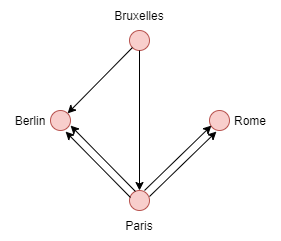
Here are some useful methods for multigraph:
| Function | Description | Return type | |---|---|---| | MultiDiGraph() | Returns a directed multigraph | MultiDiGraph | | MultiGraph.in_degree() | Returns an undirected multigraph | MultiGraph |
import networkx as nx
directed_multi_graph = nx.MultiDiGraph()
undirected_multi_graph = nx.MultiGraph()
V = {'Dublin', 'Paris', 'Milan', 'Rome'}
E = [('Milan','Dublin'), ('Milan','Dublin'), ('Paris','Milan'), ('Paris','Dublin'), ('Milan','Rome'), ('Milan','Rome')]
directed_multi_graph.add_nodes_from(V)
undirected_multi_graph.add_nodes_from(V)
directed_multi_graph.add_edges_from(E)
undirected_multi_graph.add_edges_from(E)
## Weighted Graphs
A weighted graph (**G**) is defined by a set of vertices (**V**) and edges (**E**) or links interconnecting the vertices, and including a weighted function that assigns a number as a weight to each edge.
Thus, we can say that a weighted graph is mathematically represented as: **G = (V,E, w)** where V is represented by a set of vertices **V={ V1, .., Vn}** which are connected by a set of edges defining the links between each vertex **E= {{Vk, Vi} ... {Vi,Vn}}** and whose edges have a weighted function assigning a weight w: V -> R.
Note:
* If E is a set of ordered couples: oriented weighted graph
* If E is a set of two sets: unoriented weighted graph
* If E is a multiset: weighted multigraph (directed weighted multigraph)
* If E is a set of ordered couples: oriented weighted graph
**Example**
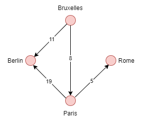
The weight of an edge is estimated as the cost to reach a vertex. In this case, for Brussels to reach Berlin, it would cost 11.
import networkx as nx
G = nx.DiGraph()
V = {'Dublin', 'Paris', 'Milan', 'Rome'}
E = [('Milan','Dublin', 19), ('Paris','Milan', 8), ('Paris','Dublin', 11), ('Milan','Rome', 5)]
G.add_nodes_from(V)
G.add_weighted_edges_from(E)
## Bipartite Graphs
These are multipartite graphs such as bipartite, tripartite, or kth-partite graphs, which are graphs whose vertices can be partitioned into two, three, or Xth set of vertices.
Use cases:
* When processing documents and structuring information into a bipartite graph of documents and entities that appear in the documents.
* When dealing with transactional data to encode relationships between buyers and merchants.
**Example**
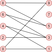
import networkx as nx
import pandas as pd
import numpy as np
n_nodes = 10
n_edges = 12
bottom_nodes = [ith for ith in range(n_nodes) if ith % 2 ==0]
top_nodes = [ith for ith in range(n_nodes) if ith % 2 ==1]
iter_edges = zip(
np.random.choice(bottom_nodes, n_edges),
np.random.choice(top_nodes, n_edges))
edges = pd.DataFrame([
{"source": a, "target": b} for a, b in iter_edges])
B = nx.Graph()
B.add_nodes_from(bottom_nodes, bipartite=0)
B.add_nodes_from(top_nodes, bipartite=1)
B.add_edges_from([tuple(x) for x in edges.values])
## adjacency matrix
An adjacency matrix provides a better representation of a graph. Thus, a matrix M of a graph G = (V, E) is a square matrix of vertices (|V| x |V|) such that Mij is equal to 1 if there is an edge from I to J and 0 otherwise.
**Example**
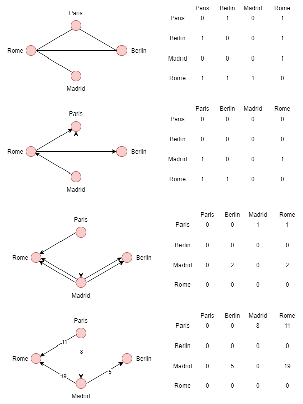
* For non-oriented graphs, the weight applies to each of the vertices.
* For oriented graphs (bigraphs), the weight applies to the starting vertex.
* For multigraphs, the value changes when multiple edges point to the same vertex.
* For weighted graphs, each matrix value has a higher weight depending on the weight defined by the edge.
## metrics
Each graph represents a network of a given size by: the number of vertices and edges. But this data is not enough for this, there are 4 types of metrics:
* **Integration Metrics**: Measures how each vertex is interconnected with each other
* **Segregation Metrics**: Quantifies the presence of groups of vertices that are connected to each other (modules)
* **Centrality Metrics**: Evaluates the importance of individual vertices
* **Resilience Metrics**: Measures a network's ability to maintain and adapt its operational performance in the face of failures.
### Integration Metrics
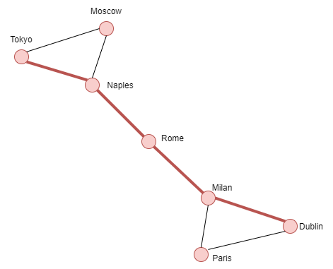
Let's talk about the concept of distance: it is linked to the number of edges to travel to reach a given vertex. We have therefore:
* A starting vertex I
* An arrival vertex J
* The shortest path (the set of edges between the two vertices) (fewer edges).
* The diameter (the number of edges in the shortest path)
**Shortest Path**
| Function | Description | Return Type |
|---|---|---|
| shortest_path(Graph, Number source, Number target) | Returns the shortest path in a graph | Array |
Example:
```python
import networkx as nx
G = nx.Graph()
nodes = {1:'Dublin',2:'Paris',3:'Milan',4:'Rome',5:'Naples',
6:'Moscow',7:'Tokyo'}
G.add_nodes_from(nodes.keys())
G.add_edges_from([(1,2),(1,3),(2,3),(3,4),(4,5),(5,6),(6,7),(7,5)])
path = nx.shortest_path(G,source=1,target=7)
Result:
[1,3,4,5,6]
**Length of the path**
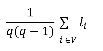
To calculate the length of the path:
* Li is the average length of the path between 2 nodes
* V is the set of vertices
* q = |V| represents the order
| Function | Description | Return Type |
|---|---|---|
| average_shortest_path_length(Graph) | Returns the length of the path | Float |
Note: It is not always possible to calculate a path among all vertices that are not connected.
import networkx as nx
nx.average_shortest_path_length(G)
Result:
2.1904761904761907
**Global and Local Efficiency** The global efficiency is the average of the inverse of the shortest path length for all edges. Thus:
* Lij is the shortest path between vertex i and j
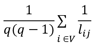
The local efficiency of a node can be calculated by considering only the neighborhood of the node in the calculation.
| Function | Description | Return Type |
|---|---|---|
| global_efficiency(Graph) | Returns the length of the path | Float |
| local_efficiency(Graph) | Returns the length of the path | Float |
import networkx as nx
nx.global_efficiency(G)
nx.local_efficiency(G)
Result:
0.6111111111111109
0.6666666666666667
In conclusion, we can say that a fully connected graph is more efficient than a circular graph. In fact, in a fully connected graph, each vertex reaches its goal more quickly by using other vertices, whereas a circular graph needs to pass through all other vertices.

### Segregation Metrics
**Clustering Coefficient**
Measures the number of clustered vertices. It is defined as triangles (3 vertices and three edges) around a vertex and is equivalent to the fraction of neighboring vertices.
| Function | Description | Return Type |
|---|---|---|
| average_clustering(Graph) | Returns the average of the neighborhood | Float |
| clustering(Graph) | Returns the neighborhood | Object |
import networkx as nx
nx.average_clustering(G)
nx.clustering(G)
Result:
0.6666666666666667
{1: 1.0,
2: 1.0,
3: 0.3333333333333333,
4: 0,
5: 0.3333333333333333,
6: 1.0,
7: 1.0}
**Modularity**
Quantifies the division of a network into a set of interconnected vertices (or modules, clusters, etc.). The main idea is that networks with high modularity will display dense connections within the module and sparse connections between modules.
Consider a social network such as Reddit: members of communities related to video games tend to interact much more with other users in the same community, discussing the latest news, favorite consoles, etc. However, they will likely interact less with users who talk about fashion. Unlike many other graph metrics, modularity is often calculated using optimization algorithms.
Segregation measures help understand the presence of groups. However, each vertex in a graph has its own importance. To quantify this, we can use centrality metrics.
| Function | Description | Return Type |
|---|---|---|
| modularity(Graph, Array communities) | Returns the modularity | Float |
Communities is a list of sets, each representing a partition of the graph.
import networkx.algorithms.community as nx_comm
nx_comm.modularity(G, communities=[{1,2,3}, {4,5,6,7}])
Result:
0.3671875
### Centrality Metrics
**Node Centrality** This centrality is related to the degree of a vertex, measuring the number of edges on a certain vertex. The more a vertex is connected to another, the more its centrality degree will increase.
| Function | Description | Return Type |
|---|---|---|
| degree_centrality(Graph) | Returns the centrality of each vertex | Object |
import networkx as nx
nx.degree_centrality(G)
Result:
{1: 0.3333333333333333, 2: 0.3333333333333333, 3: 0.5, 4: 0.3333333333333333, 5: 0.5, 6: 0.3333333333333333, 7: 0.3333333333333333}
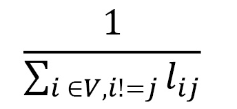
**Closeness Centrality** This metric quantifies how close a vertex is to another:
* I represents the average distance between other vertices
* V is the set of vertices
* If Lij is the shortest path between i and j, the centrality is defined as:
| Function | Description | Return Type |
| --- | --- | --- |
| closeness_centrality(Graph) | Returns the closeness of each vertex | Object |
import networkx as nx
nx.closeness_centrality(G)
Result:
{1: 0.4, 2: 0.4, 3: 0.5454545454545454, 4: 0.6, 5: 0.5454545454545454, 6: 0.4, 7: 0.4}
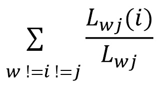
**Betweenness Centrality** measures the extent to which a vertex acts as a bridge between other vertices in the graph, meaning that even poorly connected vertices can be connected.
* Lwj is the total number of shortest paths between w and j.
* Lwj(i) is the total number of shortest paths between w and j, but passing through i.
| Function | Description | Return Type |
| --- | --- | --- |
| betweenness_centrality(Graph) | Returns the betweenness centrality of each vertex | Object |
import networkx as nx
nx.betweenness_centrality(G)
Result:
{1: 0.0, 2: 0.0, 3: 0.5333333333333333, 4: 0.6, 5: 0.5333333333333333, 6: 0.0, 7: 0.0}
### Resilience Metrics
**Assortativity Centrality** measures the tendency of vertices to be connected to similar vertices. Pearson correlation coefficient between the vertices:
* the coefficient takes positive values when there is a correlation between vertices of similar degree.
* the coefficient takes negative values when there is a correlation between vertices of different degrees.
| Function | Description | Return Type |
| --- | --- | --- |
| degree_pearson_correlation_coefficient(Graph) | Returns the assortativity centrality | float |
import networkx as nx
nx.degree_pearson_correlation_coefficient(G)
Result:
-0.6
## Practical Application
The theory is now learned, we need concrete cases to illustrate our theory.
**Fully connected undirected graph**
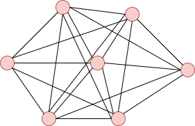
The undirected graph represents a fundamental element that can appear in larger graphs. We have a fully connected subgraph of n vertices inside a larger graph: a clique of size n.
import networkx as nx
nx.complete_graph(n=7)
A clique C is a subset of vertices c C v, such that: every two distinct vertices in the subset are adjacent. Cliques represent one of the basic concepts of graph theory and are often also used in mathematical problems where relationships need to be encoded.
**Complete Graph**:
It is a fully connected graph.
**Lollipop Graph**:
It forms a clique of size n and a branch of m vertices.
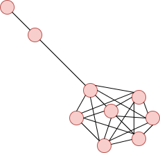
import networkx as nx
nx.lollipop_graph(m=7, n=3)
**Barbell Graph**:
Formed by two cliques of size m1 and m2 connected by a branch of vertices.
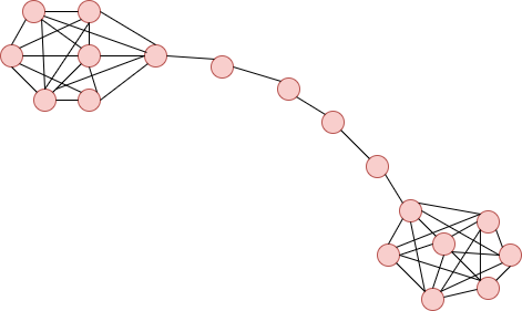
import networkx as nx
nx.barbell_graph(m1=7, m2=4)
These simple graphs are basic building blocks that can be used to generate more complex networks by combining them.

 English
