Introduction

Gradient descent is an algorithm that can be used to find the values of w and b that result in the smallest possible cost, j, for linear regression. It is commonly used in machine learning, not only for linear regression, but also for training more advanced models such as deep learning models. Understanding gradient descent is a crucial building block in machine learning.

Explanation of gradient

To create a gradient, we have the cost function j of w : 𝐽(𝑤,𝑏), that we want to minimize. 𝐽(𝑤,𝑏): is a function called for linear regression. Gradient descent is not limited to linear regression and can be applied to a wide range of cost functions and models that have more than two parameters.

For example :

We have a cost function : 𝐽(W1, W2,...Wn,𝑏), you objective is to minimize J over the paramethers. Gradient descent is an algorithm that can be used to minimize a cost function, 𝐽, by finding the optimal values for the parameters (W1, W2, ..., Wn) and b. The algorithm starts with initial guesses for these parameters, which can be arbitrary. For linear regression, it is common to set the initial values of the parameters to 0.

The gradient descent algorithm adjusts the parameters (W1, W2, ..., Wn) and b iteratively in order to minimize the cost function, j. The algorithm continues to update the parameters until the cost reaches a minimum or a near-minimum point. It's worth noting that for some functions, there may be multiple minimum points, not just one. Meaning that we have more possibilties than one done by linear regression.

How to implement ?

Gradient descent is an algorithm for finding values of parameters w and b that minimize the cost function J. The gradient descent algorithm updates the parameters on each step by subtracting a small amount, determined by the learning rate alpha, from the current value of the parameter. This small amount is calculated as the derivative of the cost function with respect to the parameter, multiplied by the learning rate. More formally, on each step, the parameter w is updated to the old value of w minus alpha times the derivative of the cost function J with respect to w. We can formulate the learning rate as : the control how big of a step we will take when parameters, W and B are updated.

Keep in mind that the assignment operator encoding (that you use everyday when coding) is different than truth assertions in mathematics.

In programming, the equality operator is often represented as "==" (e.g. in Python), whereas in mathematical notation, the equal sign is used for both assignments and truth assertions. It is important to note that, in mathematical notation, the equal sign can have different meanings depending on context, such as assignment or comparison.

Let's speek about mathematic symbol:

α: The learning rate, denoted by alpha, is a small positive number between 0 and 1 that controls the step size of the update on each iteration of the gradient descent algorithm. It is used to balance the trade-off between the step size and the number of iteration required to reach the optimal solution. A common choice of the learning rate is 0.01.

Based on it we can say : The learning rate, or alpha, determines the step size when updating the parameters during the gradient descent algorithm. A high learning rate corresponds to larger step sizes, resulting in a more aggressive search for the optimal solution. Conversely, a low learning rate corresponds to smaller step sizes, resulting in a slower, but potentially more accurate search for the optimal solution.

We can add the derivation term, help to determine which step will be the next to take, it means the smaller possible : d/dw X 𝐽(w,b).

The learning rate alpha, along with the derivative term, determines the step size when moving downhill in the optimization process. It's important to note that the model has two parameters, w and b, and the parameter b is updated using a similar assignment operation. Keep in mind that derivatives come from calculus. B is assigned the old value of b minus the learning rate Alpha times this slightly different derivative term, d/db of J of wb.

We can consider this formula like this :

𝑤 = 𝑤−𝛼∂𝐽(𝑤,𝑏)∂𝑤

𝑏 = 𝑏−𝛼∂𝐽(𝑤,𝑏)∂𝑏

To correctly implement gradient descent, you can simultaneously update both parameters by assigning the new values to temporary variables temp_w and temp_b. These are computed by subtracting the corresponding derivative term from the current values of w and b. I observed that the pre-update value of w is used in the derivative term for b.

tmp_w = 𝑤 = 𝑤−𝛼∂𝐽(𝑤,𝑏)∂𝑤

tmp_b = 𝑏 = 𝑏−𝛼∂𝐽(𝑤,𝑏)∂𝑏

Then, the updated values are assigned back to w and b.

w = tmp_w b = tmp_b

Be carrefull to follow these steps, changing the order and not assign tmp_w and tmp_b in the same time will not be a correct implementation. It will by the way assign a wrong value, already updated, to tmp_b and will not apply the correct value !

When discussing gradient descent, it is typically assumed that the parameters are updated simultaneously. However, it is possible to update the parameters separately, but this approach is not considered the correct way to implement gradient descent and would be considered a different algorithm with different properties. It is hightly recommended to use the correct simultaneous update method.

Gradient descent intuition

To define it, and to be the more clear, let's define this graph :

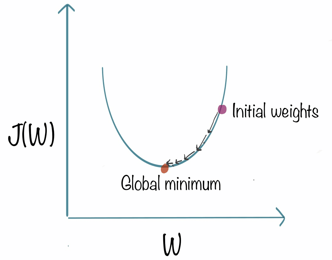
• On the horizontal axis, we have the parameter W
• On the vertical axis, we have the cost function of W

You can see that we initialized it on the initial weights, what we will do it to apply this formula :

𝑤 = 𝑤−𝛼∂𝐽(𝑤,𝑏)∂𝑤

A way to understand the derivative at a specific point on a line is to consider the tangent line that touches the curve at that point.

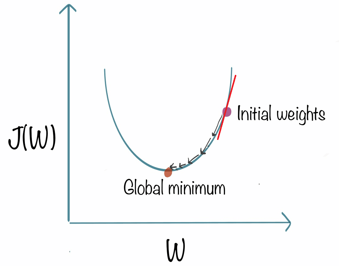
Now we have the slope of this line and it is the derivative of the function j at this point. We can define the slot by drawing like this :

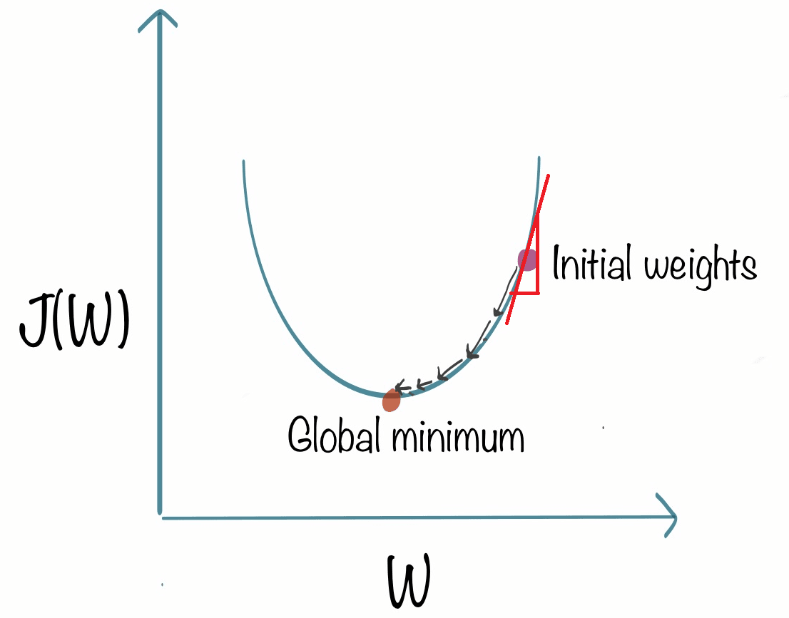
The value of the slote is : the height divided by the width of the triange. Here lets say it is 2/1, which result to positive result.

The new value for w is calculated by subtracting the product of the learning rate and a positive value from the current value of w. Since the learning rate is always positive, this results in a smaller value for w. This can be visualized as moving to the left on a graph, and as the cost J decreases as we move towards the left on the curve, this is the desired outcome as it brings us closer to the minimum value of J. Gradient descent is therefore working as intended. So lets say :

w = w - ∂ X (positive number)

The position where you will start, with this formula will always be the same in this case. The difference is : when you will start from the left of the graph, you will have this formula :

w = w - ∂ X (negative number)

Why ? because W is the point 0, going to his left means you are going to a negative value as : height equal -2 and width is 1.

When subtracting a negative number from w, it is the same as adding a positive number to w. This results in an increase of w, which can be visualized as moving to the right on a graph. As cost J decreases as we move towards the right on the curve, this is the desired outcome as it brings us closer to the minimum value of J. Thus, gradient descent is working as intended. Each case, are helping us to go closed to the minimum W value.

So when :

• We have a positive number : we decrease W
• We have a negative number: we increase W

Learning rate

The value of the learning rate, alpha, plays a crucial role in the performance of gradient descent. If alpha is not chosen properly, gradient descent may not function properly or at all. Understanding the effects of alpha can aid in selecting an appropriate value for future implementations of gradient descent. The gradient descent rule updates w as: w = w - (alpha * derivative). If the learning rate, alpha, is either too small or too large it can affect the performance of the model.

Take our formula :

𝑤 = 𝑤−𝛼∂𝐽(𝑤,𝑏)∂𝑤

To illustrate the incoming explications, we will take this image :

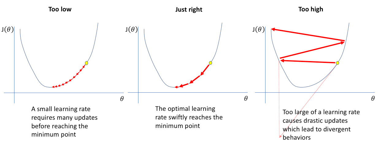
if the learning rate is too small:

When the learning rate is too small, the derivative term is multiplied by a very small number (e.g. 0.0000001) resulting in very small adjustments to the current value of w. These tiny adjustments are called "baby steps" and since the learning rate is so small, the second step is also minuscule. The result of this is that the cost J decreases, but at a very slow rate. The decrease is very slow, but will work and take a lot of time.

if the learning rate is too large:

When the learning rate is too large, the updates to w will be very large and take you far from the minimum point on the function J. Starting from a point close to the minimum, if the learning rate is too large, you take a giant step and end up at a point where the cost has actually increased.

The derivative at this new point says to decrease w, but since the learning rate is too big, you may take a huge step going from here all the way out here and overshoot the minimum again. This can result in a pattern of overshooting and never reaching the minimum. This is also known as failure to converge or even diverging. We are going further and further from the minimum, which one we will not reach

A question that may arise is what happens when one of the parameters, w, is already at a local minimum of the cost function J. If this is the case, one step of gradient descent will not change the value of w and the cost J will remain at the local minimum. Take this graph :

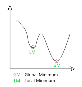
When you go to a local minimum, the slope is equal to 0, so :

w = w - ∂ * 0 or W=W.

If the value of w is 5 and ∂ is 0.1, we can consider after the first interation :

5 -0.1 * 0 = 5 So W is still equal to 5.

If the parameters have already led to a local minimum, further steps of gradient descent will not change the parameters and will keep the solution at the local minimum. This is why gradient descent can reach a local minimum even with a fixed learning rate alpha, as additional steps will not change the solution.

As we get closer to a local minimum, gradient descent will automatically take smaller steps. This is because as we approach the local minimum, the derivative gets smaller and therefore the update steps also get smaller. This happens even if the learning rate alpha is kept at a fixed value. This is the gradient descent algorithm, which can be used to minimize any cost function J, not just the mean squared error cost function used in linear regression.

How to apply gradient descent for linear regression

Lets group all together to allow us to train a model ! Lets recap some formula :

Linear regression model	Cost function	Gradient descent
𝑓𝑤,𝑏(𝑥(𝑖))=𝑤𝑥(𝑖)+𝑏	1/𝑚* m∑𝑖=0 * (𝑓𝑤,𝑏(𝑥(𝑖))−𝑦(𝑖))²	𝑤 = 𝑤−𝛼*∂/∂𝑤 𝐽(𝑤,𝑏) and 𝑏 = 𝑏−𝛼∂/∂𝑤 *𝐽(𝑤,𝑏)

To calcule de derivation for this : we can say that :

• 𝑤−𝛼*∂/∂𝑤 *𝐽(𝑤,𝑏) => ∂𝑤 𝐽(𝑤,𝑏) = 1/𝑚 m∑𝑖=0 * (𝑓𝑤,𝑏(𝑥(𝑖))−𝑦(𝑖))𝑥(𝑖)
• 𝑏−𝛼*∂/∂𝑤 *𝐽(𝑤,𝑏) => ∂𝑤 𝐽(𝑤,𝑏) = 1/𝑚 m∑𝑖=0 * (𝑓𝑤,𝑏(𝑥(𝑖))−𝑦(𝑖))

The process of gradient descent involves repeatedly updating the values of w and b until convergence is reached. It is important to remember that this is a linear regression model and f(x) = w * x + b. The derivative of the cost function with respect to w is represented by this expression and the derivative of the cost function with respect to b is represented by this expression. It is important to update w and b simultaneously on each step.

One limitation of gradient descent is that it can lead to a local minimum instead of a global minimum. A global minimum is the point that has the lowest possible value for the cost function J out of all possible points. You may recall the surface plot that looks like an outdoor park with hills, representing the cost function J, with the process of gradient descent appearing like a relaxing path through the hills.

Remember, depending on where you initialize the parameters (w,b), you can end up at different local minima.

When using gradient descent with a squared error cost function in linear regression, the cost function only has a single global minimum. This is because the cost function is a convex function, meaning it is bowl-shaped and cannot have any local minima other than the global minimum. This property makes gradient descent on a convex function more predictable as it will always converge to the global minimum as long as the learning rate is chosen appropriately.

So gradient descent, will allow you to find the best value to form your model and adjust it to perform.

Batch gradient descent is a specific type of gradient descent that uses all training examples on each step to update the model's parameters. The term "batch" refers to the fact that the entire dataset is used in each iteration of the optimization process.

In batch gradient descent, the model's parameters are updated by taking the average of the gradients of the loss function with respect to the parameters, calculated over the entire training dataset. This is in contrast to other forms of gradient descent, such as stochastic gradient descent, which update the parameters using only one training example at a time. "Batch" refers to the fact that the entire dataset is used to calculate the gradients on each update.

A contour plot of the cost function can show how the function behaves in relation to the parameters. When one axis (e.g. w1) has a narrow range of values (e.g. between 0 and 1) and the other axis (e.g. w2) has a large range of values (e.g. between 10 and 100), the contours of the cost function might form ovals or ellipses that are short on one side and longer on the other.

This is due to the fact that small changes to w1 can have a large impact on the estimated price and the cost function (J) because w1 is often multiplied by a large number (e.g. the size of the house in square feet).

In contrast, it takes a much larger change in w2 to change the predictions and thus small changes to w2 don't change the cost function nearly as much. This can make gradient descent inefficient and make it take a long time to find the global minimum.

Scaling the features, which means transforming the training data so that all features have a similar range of values, can help to make the contours of the cost function more symmetrical and make gradient descent converge more quickly.