Introduction

To explain how decision trees work, let's consider a running example:

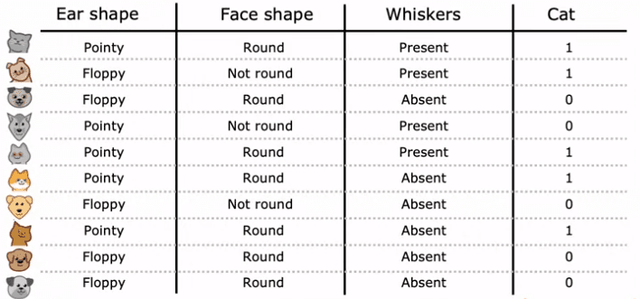
a cat classification problem. Imagine you're running a cat adoption center, and you need to classify whether an animal is a cat or not based on its features such as ear shape, face shape, and presence of whiskers. You have 10 training examples, 5 of which are cats and 5 of which are dogs. Your input features, X, are the values for ear shape, face shape, and presence of whiskers, and your target output, Y, is the label indicating whether the animal is a cat or not.

In this example, the features X take on categorical values. For instance, ear shape can be either pointy or floppy, face shape can be either round or not round, and presence of whiskers can be either present or absent. This is a binary classification task because the labels are either 1 (cat) or 0 (not cat).

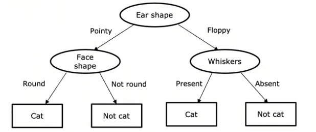
So, what is a decision tree? It's a model that is output by a decision tree learning algorithm, and it looks like a tree, with nodes and branches. If you have a new test example, you start at the root node, look at the feature written inside, and based on its value, go left or right down the tree until you reach a leaf node, which makes a prediction.

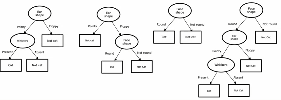
Let's consider a few examples of decision trees. In the first tree, if the ear shape of the test example is pointy, you'll look at the whiskers feature to determine whether the animal is a cat or not. In the second tree, you'll look at both the ear shape and whiskers features. The third and fourth trees are different from the first two, and some will perform better than others on the training or test sets.

Decision trees are a powerful and versatile machine learning algorithm that you can use in many applications. They are easy to understand and implement, and they can be combined with other algorithms to improve their performance. So, be sure to add them to your toolbox and start using them today!

The learning process

We'll go through the process of building a decision tree step by step. We'll use a training set of 10 examples of cats and dogs to illustrate the process.

Step 1: Choosing the Feature for the Root Node

The first step in building a decision tree is to decide what feature to use at the root node, the first node at the top of the decision tree. An algorithm is used to make this decision, which we'll discuss in more detail in a future article. For the purpose of this example, let's say that we choose the ear shape feature to be the feature at the root node.

Step 2: Splitting the Training Examples

Once we've decided on the feature to use at the root node, we split the training examples into two subsets based on the value of the ear shape feature. For this example, we'll split the 10 training examples into two groups of five - one group for pointy ears and one group for floppy ears.

Step 3: Choosing the Feature for the Left Branch

Next, we'll focus on the left branch of the decision tree and decide what feature to use to split the examples with pointy ears. Again, we'll use an algorithm to make this decision, which we'll discuss in the future. For this example, let's say we choose the face shape feature.

Step 4: Splitting the Left Branch

We then split the five examples with pointy ears into two subsets based on the face shape feature. We end up with four examples with round faces on the left and one example with a non-round face on the right. As all four examples on the left are cats, we can create a leaf node that predicts "cat."

Step 5: Creating the Right Branch

Next, we'll repeat the same process on the right branch of the decision tree, focusing on the five examples with floppy ears. Let's say we choose the whiskers feature to split these examples. After splitting the examples based on the presence or absence of whiskers, we end up with one example on the left that is a cat and four examples on the right that are not cats. We can create leaf nodes that predict "cat" on the left and "not cat" on the right.

Step 6: Evaluating the Results

Throughout this process, there were a few key decisions we had to make. The first was choosing what feature to use to split the examples at each node. We had to decide whether to split on the ear shape, face shape, or whiskers feature, based on which feature would result in the greatest "purity" of the labels. Purity in this context refers to having subsets of the data that are as close as possible to being either all cats or all dogs.

In the next article, we'll discuss entropy, which is used to estimate impurity and to minimize it. By minimizing impurity, we can get to a highly pure subset of examples, which allows us to make accurate predictions.

In conclusion, building a decision tree is a process that involves several key decisions. By understanding the steps involved and the decisions that need to be made, you can gain a deeper understanding of how decision trees work and how they can be used to make predictions.

Measuring purity

Entropy is a fundamental concept in machine learning that helps us measure the impurity of a set of data. This measure is particularly useful when building decision trees.

Imagine we have a set of six examples consisting of three cats and three dogs. We define p_1 as the fraction of examples that are cats (labeled as "one").

In this example, p_1 is equal to 3/6, or 0.5. To measure the impurity of this set, we use the entropy function, denoted as H(p_1).

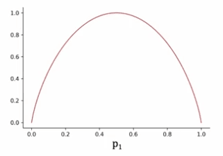
The entropy function is plotted on a graph with the horizontal axis representing p_1 and the vertical axis representing the value of the entropy.

When p_1 is 0.5, the entropy is at its highest, which is equal to one, meaning that the set is the most impure. If all the examples in the set are cats or all the examples are dogs, the entropy is zero, meaning that the set is pure.

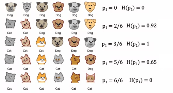
Let's take another example where we have five cats and one dog, giving us p_1 equal to 5/6 or 0.83. The entropy of p_1 is about 0.65. Another example with six cats has a p_1 of six out of six, meaning the entropy is zero. This demonstrates that as the fraction of positive examples (in this case, cats) increases, the impurity decreases, and the set becomes pure.

On the other hand, a set with two cats and four dogs has a p_1 of 2/6 or 1/3, with an entropy of 0.92. This set is more impure compared to the set with five cats and one dog, because it is closer to a 50-50 mix. A set of all six dogs has a p_1 of zero and an entropy of zero, meaning that the set is pure.

The actual equation for the entropy function is defined as negative p_1log_2(p_1) - p_0log_2(p_0), where p_0 is equal to 1 - p_1. The entropy function starts from zero, goes up to one, and then comes back down to zero as the fraction of positive examples in the sample increases. The entropy function is similar to the logistic loss in machine learning, but that is a topic for another discussion.

The entropy function is an important tool for measuring the impurity of a set of data. It is crucial for building decision trees and is defined as a function of the fraction of positive examples in a sample.

Choosing a split

When constructing a decision tree, the goal is to choose the feature that will split the data into subsets that are as pure as possible. This is done by calculating the information gain of each feature, which represents the reduction in entropy that results from splitting the data based on that feature.

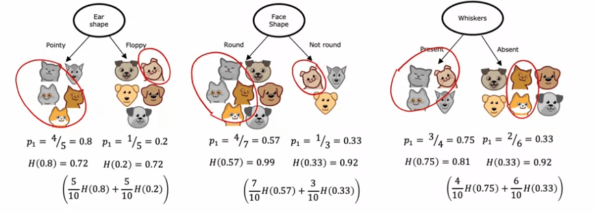
For instance, if we are building a decision tree to recognize cats and non-cats, we may have three features to choose from at the root node: ear shape, face shape, and whiskers. To decide which feature to use, we calculate the information gain of each feature, taking into account the number of examples in each of the resulting subsets.

Let's take the ear shape feature as an example. If we split on this feature, we would end up with two subsets, one containing four cats out of five examples and the other containing one cat out of five examples. The entropy of each subset can be calculated using the entropy formula, which measures the impurity of the data. In this case, the entropy of both subsets turns out to be 0.72.

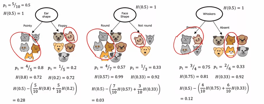
We can repeat this process for the other two features, calculating the entropy of the resulting subsets. The feature with the lowest weighted average entropy will be chosen as the feature to split on at the root node.

Note that in decision tree building, the reduction in entropy is usually expressed as a reduction compared to the entropy of the original data set, rather than as a weighted average. But either way, the goal is to choose the feature that results in the lowest entropy, thereby maximizing the purity of the resulting subsets.

Combine measuring and split

The process of building a decision tree starts with all the training examples at the root node. Then, the algorithm calculates the information gain for all the possible features, and the feature with the highest information gain is selected to split on. This split is then used to create left and right branches of the tree, and the training examples are sent to either the left or the right branch based on the value of that feature for that example.

The splitting process continues on the left and right branches of the tree, until the stopping criteria is met. The stopping criteria can be different for different implementations of the decision tree algorithm, but common stopping criteria include:

• When a node is 100% a single class
• When the entropy of the data at the node is zero
• When the maximum depth of the tree has been reached
• When the information gain from additional splits is less than a threshold
• When the number of examples in a node is below a threshold

The building process of a decision tree can also be viewed as a recursive algorithm, as the way you build a decision tree at the root node is by building other smaller decision trees in the left and right sub-branches. The way the algorithm builds these sub-decision trees is by repeating the process of calculating the information gain for all possible features and splitting the data accordingly, until the stopping criteria are met.

Using one-hot encoding of categorical features

In this section, we will explore how to handle features that can take on more than two values in machine learning. Our previous examples had features such as ear shape, face shape, and whiskers that could only take on two possible values, either pointy or floppy, round or not round, and present or absent, respectively.

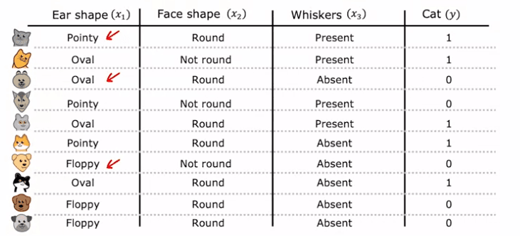
However, what if a feature such as ear shape can take on three possible values: pointy, floppy, or oval? To address this issue, we will use a technique called one-hot encoding.

One-hot encoding involves replacing a categorical feature with k binary features, where k is the number of possible values for the original feature. In this case, k is 3 for the ear shape feature. So, instead of having one feature for ear shape, we will create three new features, one for pointy ears, one for floppy ears, and one for oval ears. Each of these features can only take on two possible values, 0 or 1, and exactly one of them will have a value of 1, hence the name one-hot encoding.

With this approach, we are back to the original setting where each feature can only take on two values. The decision tree learning algorithm can be applied to this data without any modifications. The technique of one-hot encoding can also be applied to other types of machine learning models, such as neural networks.

One-hot encoding is a technique that enables decision trees and other machine learning models to work with features that can take on more than two values. By converting categorical features into a set of binary features, the machine learning algorithm can be fed with inputs that are numbers instead of categorical values.

Continuous valued features

We will explore how to modify the decision tree algorithm to work with features that are not just binary values but continuous values, meaning features that can take on any number. To illustrate this, let's use a modified version of the cat adoption center dataset that includes a new feature: the weight of the animal in pounds. This feature is useful in deciding if an animal is a cat or not.

To incorporate this feature into the decision tree learning algorithm, we must consider splitting on the weight feature along with the other features such as ear shape, face shape, and whiskers. To determine how to split on the weight feature, we need to consider many different threshold values and choose the one that results in the highest information gain.

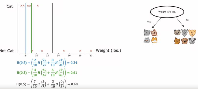
For example, if we consider splitting the data based on whether the weight is less than or equal to 8, we will split the data into two subsets. We then calculate the information gain by computing the entropy at the root and subtracting the entropy of the two subsets. However, we should try other values as well and choose the one that gives the highest information gain.

In general, we sort the examples according to the value of the feature and choose the midpoints between the sorted list of examples as the possible threshold values to consider. For each threshold value, we calculate the information gain and choose the threshold that gives the highest information gain. If the information gain from splitting on the continuous value feature is better than that from splitting on any other feature, then we choose to split at that feature.

To summarize, to make the decision tree work with continuous value features, we try different threshold values, carry out the usual information gain calculation, and split on the continuous value feature if it gives the highest possible information gain. This way, the decision tree can handle continuous value features and make predictions based on them.

Implementation of a decision three

We will use one-hot encoding to encode the categorical features. They will be as follows:

• Ear Shape: Pointy = 1, Floppy = 0
• Face Shape: Round = 1, Not Round = 0
• Whiskers: Present = 1, Absent = 0
• Therefore, we have two sets:

X_train: for each example, they contain 3 features:

  - Face Shape (1 if round, 0 otherwise)
  - Ear Shape (1 if pointy, 0 otherwise)
  - Whiskers (1 if present, 0 otherwise)

y_train: whether the animal is a cat

  - 1 if the animal is a cat
  - 0 otherwise

 import pandas as pd
import numpy as np
import matplotlib.pyplot as plt
from utils import *

X_train = np.array([[1, 1, 1],
[0, 0, 1],
 [0, 1, 0],
 [1, 0, 1],
 [1, 1, 1],
 [1, 1, 0],
 [0, 0, 0],
 [1, 1, 0],
 [0, 1, 0],
 [0, 1, 0]])

y_train = np.array([1, 1, 0, 0, 1, 1, 0, 1, 0, 0])

#For instance, the first example
X_train[0]

The output should be :

 array([1, 1, 1])

The first instance has a sharp ear shape, circular facial shape and is equipped with whiskers.

Regarding the nodes, we calculate the information gain for every feature, then split the node based on the feature with the highest information gain. This is achieved by evaluating the node's entropy against the weighted entropy of the two resulting split nodes.

It's important to note that the root node encompasses all the animals in our data set, with 𝑝𝑛𝑜𝑑𝑒1 representing the proportion of positive class (cats) in the root node.

𝑝𝑛𝑜𝑑𝑒1=5/10=0.5

This is the formula to put in place :

𝐻(𝑃𝑛𝑜𝑑𝑒1) = −𝑃𝑛𝑜𝑑𝑒1 log2(𝑃𝑛𝑜𝑑𝑒1) − (1 − 𝑃𝑛𝑜𝑑𝑒1) log2(1 − 𝑃𝑛𝑜𝑑𝑒1)

 def entropy(p):
    if p == 0 or p == 1:
        return 0
    else:
        return -p * np.log2(p) - (1- p)*np.log2(1 - p)
    
print(entropy(0.5))

To clarify, let's calculate the information gain by splitting the node for each of the features. To accomplish this, we will write some functions.

 def split_indices(X, index_feature):
    """Given a dataset and a index feature, return two lists for the two split nodes, the left node has the animals that have 
    that feature = 1 and the right node those that have the feature = 0 
    index feature = 0 => ear shape
    index feature = 1 => face shape
    index feature = 2 => whiskers
    """
    left_indices = []
    right_indices = []
    for i,x in enumerate(X):
        if x[index_feature] == 1:
            left_indices.append(i)
        else:
            right_indices.append(i)
    return left_indices, right_indices
    
split_indices(X_train, 0)

We should have as result :

([0, 3, 4, 5, 7], [1, 2, 6, 8, 9])

Now, we need to create another function to calculate the weighted entropy in the split nodes. As previously discussed, we need to determine:

• 𝑤left and 𝑤right, the proportion of animals in each node.
• 𝑝left and 𝑝right, the proportion of cats in each split.

It's crucial to distinguish between these two definitions. To give an example, if we split the root node based on the feature of index 0 (Ear Shape), the left node will contain animals 0, 3, 4, 5, and 7. The following values would then apply:

• 𝑤left = 5/10 = 0.5
• 𝑝left = 4/5 = 0.8
• 𝑤right = 5/10 = 0.5
• 𝑝right = 1/5 = 0.2

 def weighted_entropy(X,y,left_indices,right_indices):
    """
    This function takes the splitted dataset, the indices we chose to split and returns the weighted entropy.
    """
    w_left = len(left_indices)/len(X)
    w_right = len(right_indices)/len(X)
    p_left = sum(y[left_indices])/len(left_indices)
    p_right = sum(y[right_indices])/len(right_indices)
    
    weighted_entropy = w_left * entropy(p_left) + w_right * entropy(p_right)
    return weighted_entropy
    
left_indices, right_indices = split_indices(X_train, 0)
weighted_entropy(X_train, y_train, left_indices, right_indices)

Result : 

0.7219280948873623

Therefore, the weighted entropy in the two split nodes is 0.72. To calculate the Information Gain, we subtract this value from the entropy in the node we selected to split (in this case, the root node).

 def information_gain(X, y, left_indices, right_indices):
    """
    Here, X has the elements in the node and y is theirs respectives classes
    """
    p_node = sum(y)/len(y)
    h_node = entropy(p_node)
    w_entropy = weighted_entropy(X,y,left_indices,right_indices)
    return h_node - w_entropy
    
information_gain(X_train, y_train, left_indices, right_indices)

Result: 0.2780719051126377

Now, let's compute the information gain if we split the root node for each feature:

 for i, feature_name in enumerate(['Ear Shape', 'Face Shape', 'Whiskers']):
    left_indices, right_indices = split_indices(X_train, i)
    i_gain = information_gain(X_train, y_train, left_indices, right_indices)
    print(f"Feature: {feature_name}, information gain if we split the root node using this feature: {i_gain:.2f}")
    
Result:

Feature: Ear Shape, information gain if we split the root node using this feature: 0.28
Feature: Face Shape, information gain if we split the root node using this feature: 0.03
Feature: Whiskers, information gain if we split the root node using this feature: 0.12

Thus, the best feature to split is the Ear Shape. The code below demonstrates the split in action. It is not necessary to have a deep understanding of this code block.

 tree = []
build_tree_recursive(X_train, y_train, [0,1,2,3,4,5,6,7,8,9], "Root", max_depth=1, current_depth=0, tree = tree)
generate_tree_viz([0,1,2,3,4,5,6,7,8,9], y_train, tree)

Result:

 Depth 0, Root: Split on feature: 0
 - Left leaf node with indices [0, 3, 4, 5, 7]
 - Right leaf node with indices [1, 2, 6, 8, 9]

The process is iterative, meaning we repeat these calculations for each node until a stopping criteria is met, such as:

• If the tree depth after splitting exceeds a specified limit
• If the resulting node only contains instances of one class
• If the information gain from splitting is below a certain threshold.

The final tree would look similar to the diagram shown.

 tree = []
build_tree_recursive(X_train, y_train, [0,1,2,3,4,5,6,7,8,9], "Root", max_depth=2, current_depth=0, tree = tree)
generate_tree_viz([0,1,2,3,4,5,6,7,8,9], y_train, tree)

Result: 

 Depth 0, Root: Split on feature: 0
- Depth 1, Left: Split on feature: 1
  -- Left leaf node with indices [0, 4, 5, 7]
  -- Right leaf node with indices [3]
- Depth 1, Right: Split on feature: 2
  -- Left leaf node with indices [1]
  -- Right leaf node with indices [2, 6, 8, 9]

Three ensembles

One of the drawbacks of using a single decision tree is its susceptibility to small changes in the data. To overcome this weakness and make the model more robust, a tree ensemble can be used. A tree ensemble refers to the creation of multiple decision trees instead of just one.

For example, if a single decision tree is used to classify cats and non-cats, small changes in the data can result in a completely different tree being generated. This lack of robustness is why tree ensembles are often more accurate than single decision trees.

To classify a new test example, the ensemble of trees is used by running the test example through each tree and taking a majority vote on the predictions made by each tree. The final prediction is the one that receives the majority of the votes. This approach makes the overall algorithm less sensitive to the predictions made by any single tree and therefore, more robust.

We'll explore the technique of sampling with replacement, which is a key method used to build the ensemble of trees.

Sampling with remplacement

Sampling with replacement is a technique used in building a tree ensemble in machine learning. It involves creating multiple, slightly different training sets from the original training set. This is done by randomly selecting examples from the original set and adding them to a new set, then putting the selected example back into the original set and repeating the process until the new set has the desired number of examples. Some examples from the original set may be repeated in the new set and some may not be included at all. This process allows for the creation of new training sets that are similar, yet different from the original set, which is important in building an ensemble of trees.

Random forest algorithm

In this section, we will discuss the Random Forest algorithm, a powerful tree ensemble algorithm that outperforms a single decision tree. The Random Forest algorithm is created by building multiple decision trees on different training sets generated using a technique called "sampling with replacement." Given a training set of size M, the algorithm generates B new training sets by randomly selecting M examples from the original set, with replacement. Each new training set is used to train a decision tree, leading to a total of B decision trees. The final prediction is made by having each of these trees vote on the correct answer. The number of trees, B, is typically around 100, but values ranging from 64 to 228 are also common. Setting B to a higher value does not significantly affect performance beyond a certain point.

To further improve the performance of the algorithm, a modification is made to randomize the feature choice at each node. Instead of selecting the feature with the highest information gain from all available features, a random subset of K (less than N) features is chosen, and the feature with the highest information gain from that subset is selected. This modification leads to the creation of the Random Forest algorithm, which is more robust and accurate than a single decision tree.

The Random Forest algorithm explores small changes to the training set through the sampling with replacement procedure, averaging over all of those changes. This makes it less likely for any change to the training set to have a significant impact on the overall output of the algorithm.

In conclusion, the Random Forest algorithm is an effective and robust machine learning technique. Although it is outperformed by another algorithm called Boosted Decision Trees, it is still a useful tool for machine learning engineers.

XGBoost

In this section, we will discuss XGBoost, the most commonly used implementation of decision tree ensembles. XGBoost is a fast and efficient open source implementation of boosted trees, which is a modification of the decision tree algorithm. Boosting focuses on the examples that the previous decision trees in the ensemble misclassified, allowing the algorithm to learn more quickly.

To implement boosting, the algorithm looks at the decision trees trained so far and determines which examples are still being misclassified. On each iteration, a higher probability is given to picking examples that the ensemble is still not doing well on, focusing the attention of the next decision tree in the ensemble. The mathematical details of how to increase the probability are complex, but the open source implementation of XGBoost takes care of them.

XGBoost also has built-in regularization to prevent overfitting, making it a highly competitive algorithm in machine learning competitions. Instead of using sampling with replacement, XGBoost assigns different weights to different training examples, making it even more efficient. To use XGBoost, one can simply import the library and initialize a model as an XGBoost classifier or regressor.

In conclusion, XGBoost is a powerful and widely used algorithm for decision tree ensembles. Its open source implementation is efficient and easy to use, and it has been successful in many machine learning competitions and commercial applications.

When to use decision threes

When choosing between decision trees and neural networks as machine learning algorithms, it's important to consider the type of data you're working with and the specific requirements of your task.

Decision trees and tree ensembles are a type of supervised learning algorithm that are well-suited for tabular or structured data, such as data stored in a spreadsheet format. They use a tree-like structure to make predictions based on the values of the features in the data. Decision trees are fast to train and can be interpretable, meaning that you can understand how the model is making decisions, especially for small trees with only a few dozen nodes.

However, decision trees are not as effective when working with unstructured data, such as images, video, audio, or text. Neural networks, on the other hand, are a type of artificial neural network that can handle all types of data, including structured, unstructured, and mixed data. Neural networks are typically more powerful and can achieve better performance on complex tasks, but they can be slower to train, especially for large networks. Additionally, neural networks can benefit from transfer learning, where pre-training on a larger dataset can improve the performance of the model on a smaller, related task.

In conclusion, the choice between decision trees and neural networks will depend on the type of data you're working with and the specific requirements of your task. While decision trees are fast to train and can be interpretable, they are not as effective on unstructured data. Neural networks are more powerful and can handle all types of data, but they can be slower to train. Both algorithms have their strengths and weaknesses, and the right choice will depend on the specific task at hand.