Introduction

Convolutional neural networks (CNNs) are a class of deep neural networks widely used for image recognition, computer vision, speech recognition, and natural language processing. CNNs have revolutionized the way computers process images by enabling them to recognize and classify objects in images with high accuracy. Their architecture is based on convolutional layers that automatically extract features from images, followed by subsampling layers that reduce the dimensionality of the data, and finally, classification layers that predict the class of an image. In this article, we will explore the basics of CNNs and their applications in different domains.

How it Works

Convolutional neural networks, or CNNs, are an artificial intelligence technique that allows for understanding images using an algorithm. The functioning of this technique is simple to understand.

Firstly, an image is sent into the neural network. The network processes it in multiple stages. First, it identifies the basic shapes present in the image, such as edges and angles. Then, it combines these shapes to extract more complex features, such as patterns or textures. Finally, it uses these features to determine what the image represents.

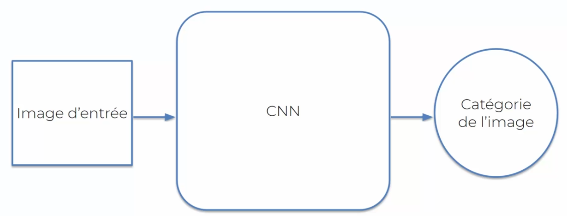
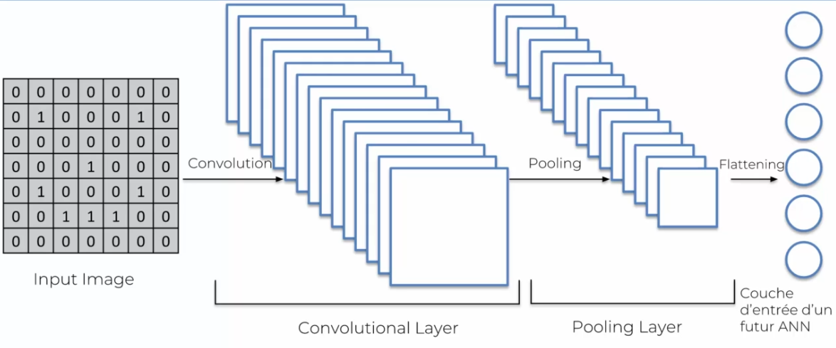
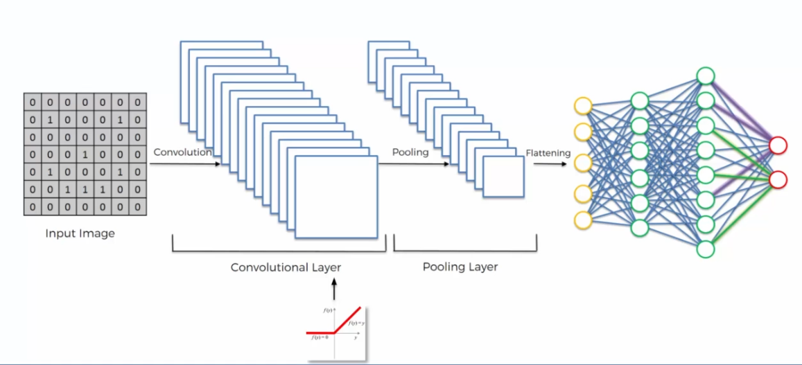
To facilitate this feature extraction, the neural network uses filters that pass over the image at different scales. These filters are the convolutional layers. Next, to reduce the size of the data and keep only the essentials, subsampling layers are used. Finally, the classification layers predict the class of the image.

For the neural network to read an image, it must first be trained. This means that we present it with images and tell it the categories to which they belong. The network then learns to recognize the features that differentiate the different categories.

Once the network has been trained, it can be used to predict the category of a new image. However, it is important to note that the predictions are not always 100% reliable. There may be errors or inaccuracies.

But how does the neural network read an image?

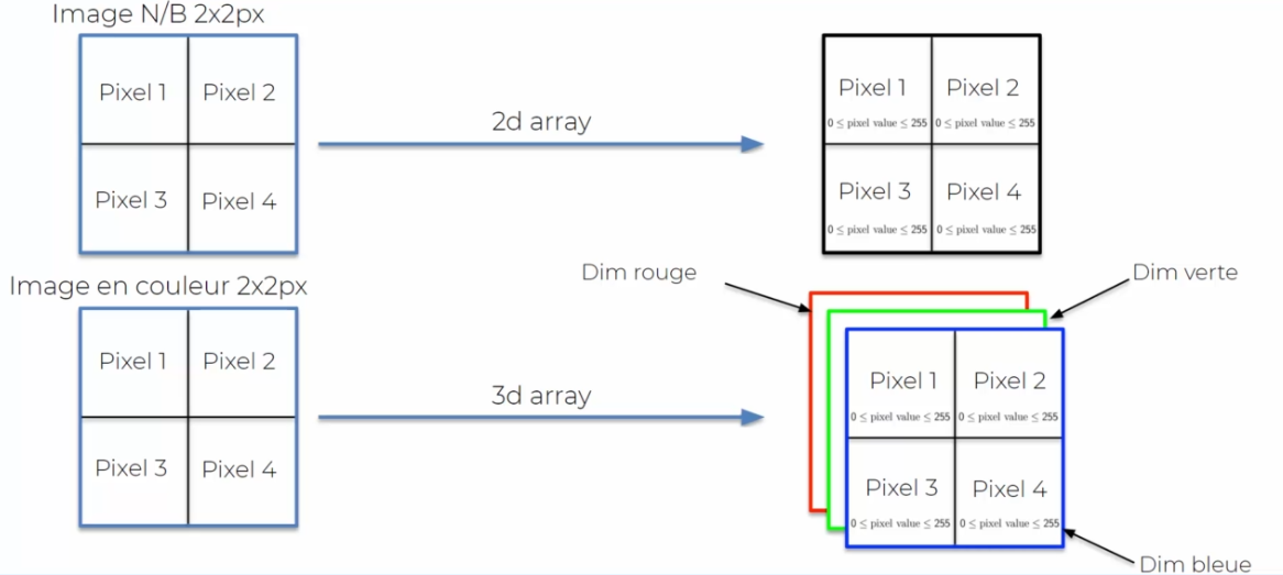
Firstly, it's important to understand that an image is composed of a cluster of pixels. Each pixel has a value from 0 to 255 for black and white, or from 0 to 255 for each color channel (red, green, and blue) in the case of a color image. The neural network can therefore read the image by breaking it down into a table of pixels. It then uses convolutional layers to identify the features of the image, such as edges, patterns, or textures. These features are then combined and used to predict the category of the image.

Convolution

Let's now consider the case of an image in pixels. As mentioned earlier, an image is a cluster of pixels:

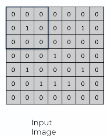
To translate an image into a string of characters, we need a feature detector. This detector will allow us to detect the features of the image that are important for classification.

The feature detector is a small array of numbers called a "filter" or "kernel." The filter is applied to the image by multiplying its values by the corresponding pixel values of the image. This operation is called "convolution."

Convolution produces a new image, called a feature map. This feature map is a representation of the image that highlights the features detected by the filter. For example, if the filter detects horizontal edges, the feature map will highlight the horizontal edges present in the image.

The feature detector can be trained on many images to detect different features. Several feature detectors can also be combined to detect more complex features.

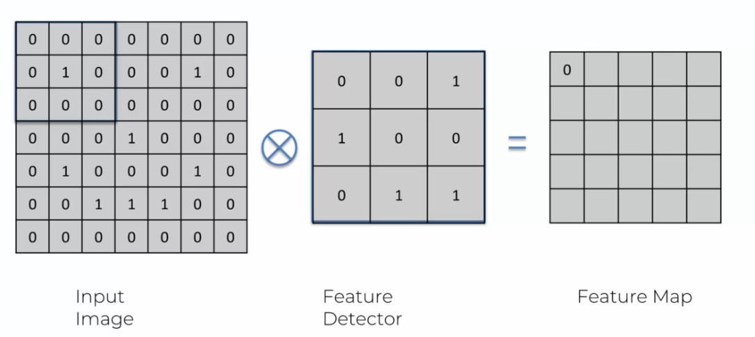
To illustrate the functioning of convolution, let's take the example of a 3x3 feature detector applied to an image of the same size.

To start convolution, we place the detector in the upper left corner of the image. We then multiply the values of the detector by the corresponding values of the image, and then add the results. This gives a single number that represents the value of this area of the image. This process is repeated for each area of the image.

If the detector doesn't detect a feature in this area of the image, the obtained value will be close to zero. If the detector detects a feature, the obtained value will be larger. This operation is repeated for each area of the image, creating a new image called a "feature map."

In the example above, if the entire feature detector is multiplied by the corresponding part of the image, the resulting response will be constantly 0. This means that this area of the image does not contain the feature that the detector is designed to find.

To continue convolution, we move the detector to the right and repeat the process. We continue to move the detector from left to right until the end of the line is reached. Then, we move the detector down one row and repeat the process. We repeat this process for each area of the image.

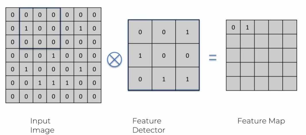
During convolution, it is possible to get multiple positive responses for the same feature. In this case, each positive response is recorded in the feature map. A mark (a 1 in the example below) is placed at each location where the feature is detected.

If multiple occurrences of the same feature are detected, the marks are added together to obtain the final value for that area of the feature map.

Of course, we can use larger detectors, but the 3X3 detector is a standard that offers good performance. It will be more time-consuming as we traverse the image, but it allows for a precise analysis of the image. At the end of our convolution in this example, we obtain the following result:

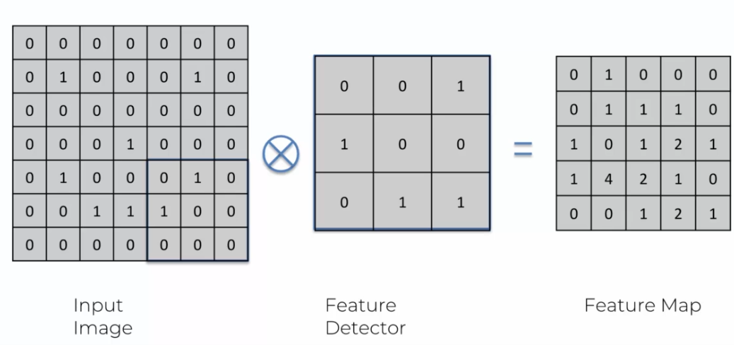
We have therefore reduced our image, which was 7X7, to 5X5, and we have created a feature map that allows us to identify the image more easily.

The Relu function

Now that we have created our feature map by applying convolution to the image, it is time to apply a rectifier function. The most commonly used function for this is the Relu function.

The Relu function is important because it makes the results of convolution nonlinear. Indeed, the contours and details of an image are not linear. The Relu function therefore allows us to accentuate them and highlight the most important features of the image.

The Relu function also removes negative values in the feature map. Negative values are often associated with black color in the image. By removing these values, the Relu function simplifies the image, making it easier to interpret by the neural network.

This mathematical function is applied to each element of the feature map produced by convolution. It is defined as follows:

$$Relu(x) = max(0,x)$$

Relu returns 0 if the input is negative and the input itself if it is positive or zero. This function has the advantage of being very simple and very fast to compute.

The Relu function also has another important advantage: it does not change the size of the feature map. Indeed, it only replaces negative values with zeros. This allows us to maintain the size of the feature map and facilitate the computation of convolution on the following layers of the neural network.

Pooling

An image can be upside down, show a person in a different position, or show a different part of the person. This may seem complicated because there are many possibilities, but our brain is capable of recognizing a person in all these situations.

For image recognition models to work, they must be able to adapt to all these situations. To do this, we use a technique called "max pooling". This technique is very similar to the convolutional step seen earlier, but always taking the maximum of the values of 2x2 squares of the feature map.

Max pooling simplifies the image while preserving important features. By taking the maximum of the values of each square, we keep the most important features of the feature map while reducing its size. This also makes the model more robust by eliminating small variations of a feature that could be due to noise in the image.

Example

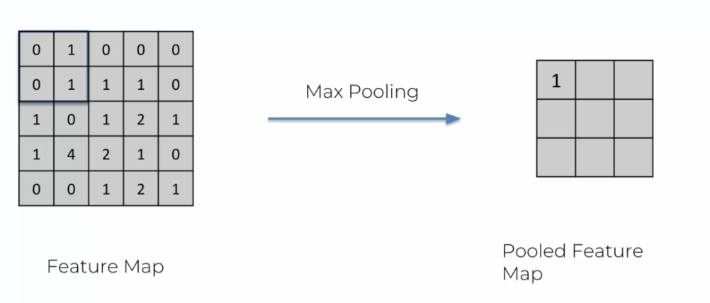
We constantly move to the right, but unlike convolution, we take a smaller matrix. When we move to the right, we do not stop to go to the next line. Instead, we read the value taking into account that we only have two elements instead of four.

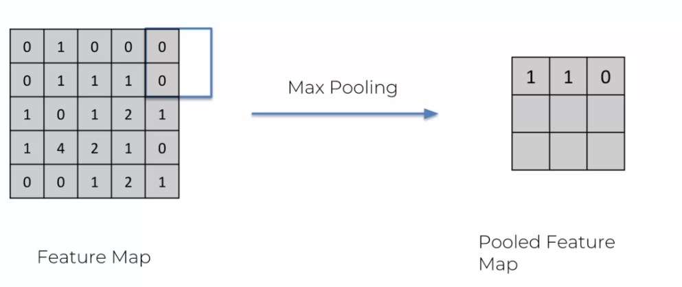
On continue alors jusqu'à obtenir une matrice totalement remplie:

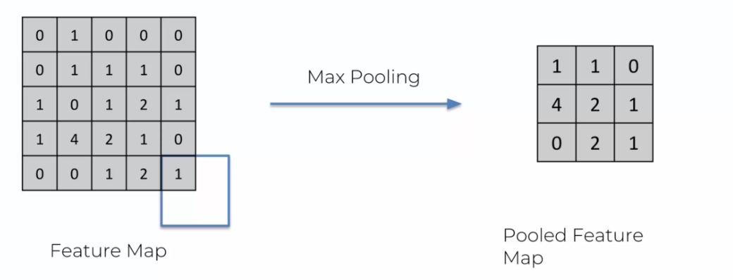
By removing information, we can see that the number of zeros decreases. However, this removed information is not necessary for our model. Indeed, it is possible to determine a face without needing to see the background scenery or to guess the person without knowing their clothes. Therefore, by removing this information, we avoid overfitting and obtain a more performant model.

Flattening Layer

The flattening layer is the simplest step to understand after pooling. It consists of flattening the matrix into a single line. This step prepares the data to be passed into the neural network.

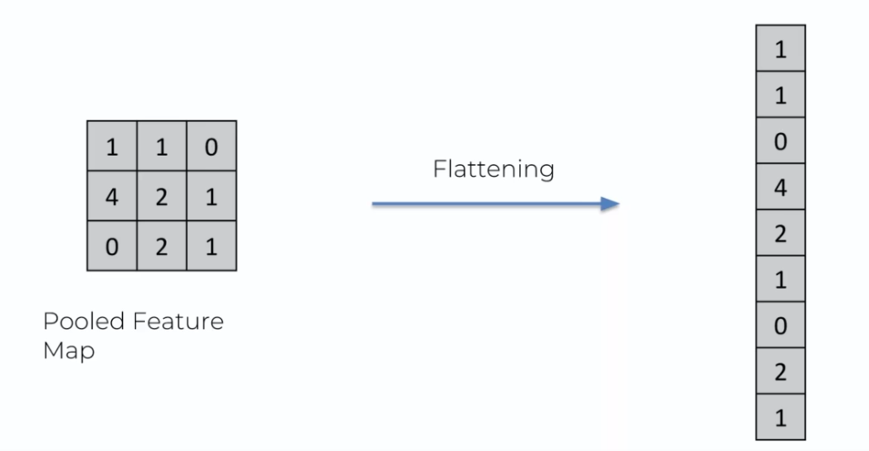
The flattening layer creates an input layer for our neural network by transforming the flattened image into a line of data. In summary, here is how our image has been translated so far into the network:

Fully Connected Layer

The last step of the image processing process is to add a fully connected neural network next to the convolutional neural network. This step is essential for image classification, as it allows the model to learn more complex features and make decisions based on these features. The fully connected neural network consists of several layers of neurons that are connected to each other. These neurons take input from the previous layer and produce outputs that are passed to the next layer. The outputs of the last layer of neurons are used for image classification based on predefined classes. Adding this fully connected neural network improves the performance of the image processing model and allows for more accurate results.

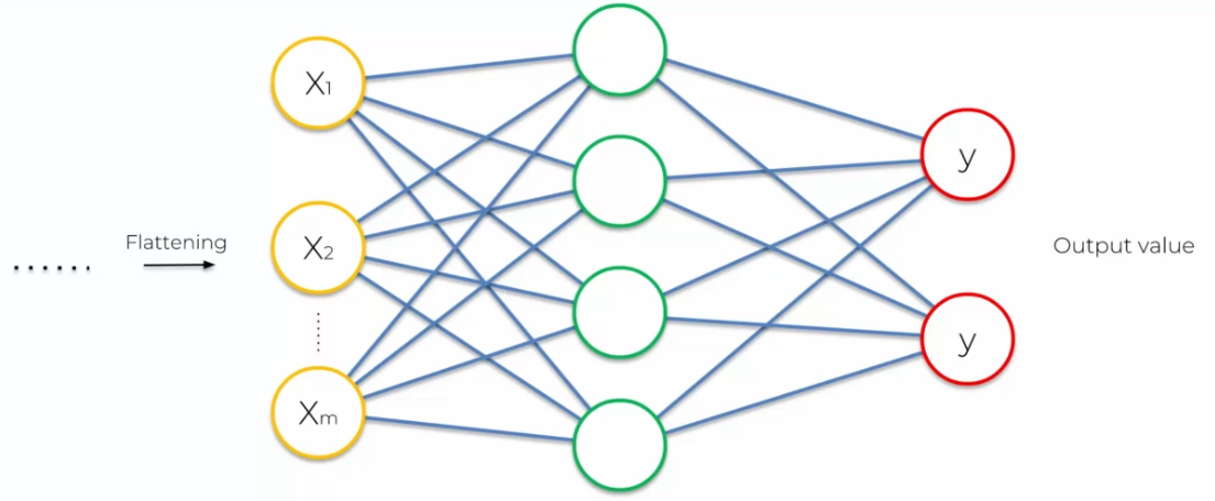
Let's take the example of an image classification model that needs to distinguish between images of cats and dogs:

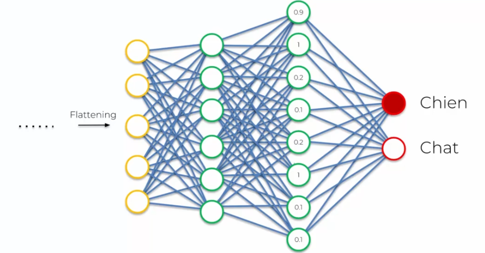
The model starts by applying convolutional filters to extract features from the images, such as edges, shapes, and textures of different parts of the image. Then, it applies a pooling function to reduce the size of the image while retaining important information.

After that, the flattening layer transforms the data into a line of values, which is then passed to the fully connected neural network. The fully connected neural network is trained to learn the features of cat and dog images by adjusting the weights of its neurons. The weights are adjusted based on the output of the model for each image, which indicates whether it is a cat or a dog.

Prompt

When the model is tested on a new image, it applies convolution filters to extract features from the image, reduces the image size with pooling, and then uses the fully connected neural network to determine whether it is a cat or a dog based on the learned features during training.

Overall, our network looks like:

Softmax Function and Cross-Entropy

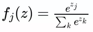
The softmax function is often used in the field of machine learning and natural language processing to convert scores from a vector into probabilities, especially for classifying data into multiple classes. The formula for the softmax function is as follows:

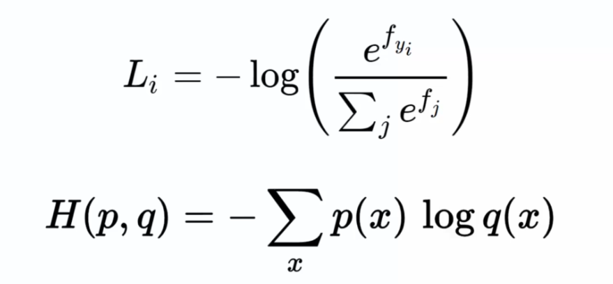
In logistic regression, when dealing with a large number of possible choices, the max-pooling function is often used, which selects the maximum value as the answer. This function is often used with cross-entropy, a commonly used cost function for measuring the difference between the actual probability distribution and the one estimated by the model. Mathematically, cross-entropy is defined as follows:

When creating a neural network, we must define a cost function that measures the gap between the model's predictions and the true values of the data. In the case of classic neural networks, the squared error is often used (difference between the actual values Y and the predictions ^Y). The goal is to minimize this cost function by adjusting the network's weights through a gradient calculation procedure.

However, for convolutional networks, cross-entropy is used as the cost function instead. Cross-entropy measures the difference between the actual probability distribution of the data and the one estimated by the model. It is particularly suited for classification problems, where each data point must be classified into one or more categories.

During the training process, the convolutional neural network uses the backpropagation method to adjust the network's weights in order to minimize the cost function. At each iteration, the network calculates the value of the cost function and adjusts the weights based on the gradient of this function with respect to the weights. This process is repeated until the cost function is sufficiently low or the maximum number of iterations is reached.

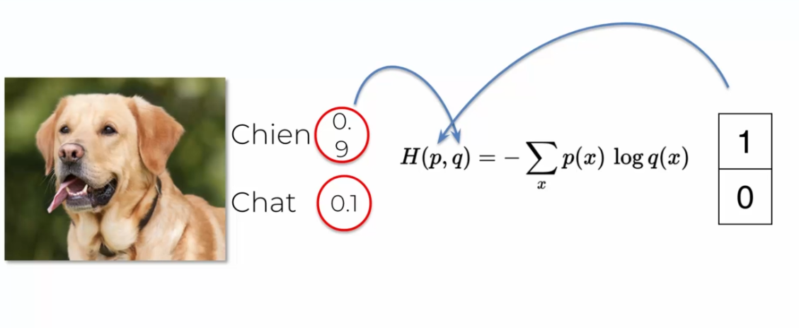
Prompt

Using cross-entropy as the cost function in convolutional neural networks has several advantages over other cost functions, such as mean squared error. One of the advantages is its ability to handle multi-class classification problems.

Let's take the example of two neural networks, NN1 and NN2, using mean squared error and cross-entropy as cost functions, respectively. Imagine that we have three images of a dog, a cat, and a weird-looking dog, and these two neural networks produce different results for the image of the weird-looking dog, with a high error for NN1 and a low error for NN2.

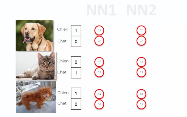
One advantage of using cross-entropy in convolutional neural networks is that it can help avoid slow convergence problems during training. If the output values are initially very small compared to the true values, using mean squared error (squared difference) can significantly slow down the learning process because the gradient will also be very small.

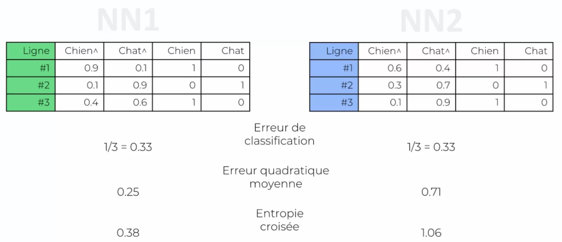
In contrast, cross-entropy takes the logarithm of the error, which means that larger errors have a more significant impact on the cost function. This allows the gradient descent algorithm to progress more quickly towards an optimal solution. Thus, using cross-entropy can improve the speed and stability of learning in convolutional neural networks.

Improving Your Network

Adding convolutional layers can improve results and reduce overfitting in convolutional neural networks. To do this, you can add a convolutional layer after pooling, which further reduces the image size. After adding the convolutional layer, it is also necessary to add a new pooling layer. It is important to note that pooling is always associated with a convolutional layer, and vice versa.

Another solution to improve results is to increase the size of the images during convolution to acquire more details. For example, you can increase the initial size from 64x64 to 150x150.

To increase the accuracy of the model, you can increase the number of training epochs. The more the model trains, the more it can learn patterns in the data.

Finally, to add more granularity to the model, you can add hidden layers. However, it is important to note that this can increase the risk of overfitting. To avoid this, you can use the dropout function, which randomly disables some connections between neurons at each training iteration, increasing the robustness of the model.