Introduction of activation functions
When building neural networks, it is common to use the sigmoid activation function in all the nodes in the hidden layers and in the output layer. However, using different activation functions can make a neural network much more powerful. In this article, we will discuss how to use different activation functions and their impact on the performance of a neural network.
Activation fonctions
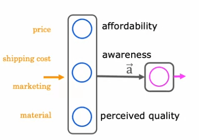
Let's consider an example of predicting the top-selling items based on factors such as price, shipping cost, marketing, and material. This example assumes that awareness of the product is binary - either people are aware or they are not. However, it is possible that the degree of awareness may not be binary and could be any non-negative number.
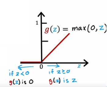
To address this, we can use a different activation function that allows for a wider range of values. A very common activation function used in neural networks is the rectified linear unit (ReLU) activation function, which is defined as g(z) = max(0, z). This function is useful because it allows for non-negative values and can better model awareness as a continuous variable.
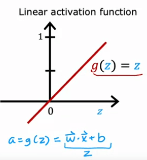
Another commonly used activation function is the linear activation function, which is defined as g(z) = z. While this function does not introduce any non-linearity, it can be useful in certain situations.
What can we think about ?
In conclusion, the choice of activation function can have a significant impact on the performance of a neural network. The sigmoid function, ReLU, and linear activation function are some of the most commonly used functions in deep learning. It's important to experiment with different activation functions to find the best one for your specific problem. Additionally, understanding the mathematics behind these functions and the impact on the neural network can help you make better decisions when designing a neural network.
How to choice ?
When considering the activation function for the output layer, it is important to consider the type of problem you are trying to solve. For example, if you are working on a binary classification problem where the target label is either zero or one, then the sigmoid activation function is often the most natural choice. This is because the neural network will learn to predict the probability that the label is equal to one, similar to logistic regression.
On the other hand, if you are solving a regression problem, such as predicting tomorrow's stock price change, then a linear activation function may be a better choice. This is because the output of the neural network can take on either positive or negative values.
For hidden layers, the most common choice of activation function is the rectified linear unit (ReLU) activation function. This is because the ReLU function is faster to compute and has been found to be effective in many situations. Additionally, the ReLU function goes flat only in one part of the graph, whereas the sigmoid activation function goes flat in two places which can slow down the training process.
The choice of activation function can have a significant impact on the performance of a neural network. It is important to experiment with different activation functions to find the best one for your specific problem. Understanding the mathematics behind these functions and the impact on the neural network can also help you make better decisions when designing a neural network.
Why do we need these activation functions ?
Neural networks are powerful machine learning models that are used to solve a variety of problems, such as image classification, natural language processing, and demand prediction. However, in order for a neural network to work effectively, it needs to have activation functions in place. An activation function is a mathematical function that is applied to the output of a neuron, which helps to introduce non-linearity into the model.
One of the most important reasons for using activation functions is that without them, a neural network would become no different than a linear regression model. This is because the linear activation function, which is represented by the equation g(z) = z, does not introduce any non-linearity into the model.
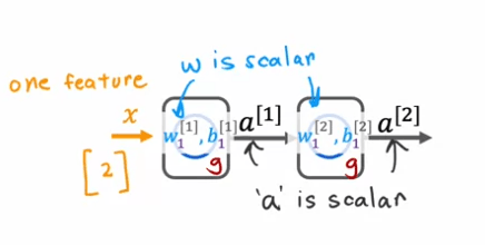
To illustrate this, let's consider a simple example of a neural network with one hidden unit and one output unit. The input x is a number, and the hidden unit has parameters w1 and b1 that output a1, which is also a number. The output unit has parameters w2 and b2 and outputs a2, which is the final output of the neural network.
If we were to use the linear activation function everywhere in this neural network, the computation of a1 would be represented by the equation a1 = g(w1x + b1), but since g(z) = z, this is equivalent to w1x + b1. Similarly, the computation of a2 would be represented by the equation a2 = g(w2a1 + b2), which simplifies to w2w1x + w2b1 + b2.
If we simplify this further, we can see that a2 is just a linear function of the input x, which means that this neural network is no different than a linear regression model. This is why having multiple layers in a neural network doesn't let the neural network compute any more complex features or learn anything more complex than just a linear function.

In general, if we were to use a linear activation function for all the hidden layers and also use a linear activation function for the output layer, then the output a4 can be expressed as a linear function of the input features x plus b. Alternatively, if we were to use a linear activation function for all the hidden layers, but use a logistic activation function for the output layer, then the model becomes equivalent to logistic regression.
In conclusion, activation functions are crucial for neural networks as they introduce non-linearity into the model, which is necessary for the neural network to be able to learn more complex features. In practice, the ReLU activation function is commonly used in hidden layers, which works well in most cases.
Multiclass
Multiclass classification is a type of classification problem where there are more than just two possible output labels. This means that instead of just having two options, such as zero or one, there can be multiple classes to choose from.
For example, in a handwritten digit classification problem, we might want to recognize all 10 digits instead of just 0 and 1. Or in medical diagnosis, we might want to classify patients with any of three or five different possible diseases. This would also be a multiclass classification problem.
In a multiclass classification problem, the output variable y can only take on a small number of discrete categories, but now y can take on more than just two possible values.
In contrast to binary classification problems, where we would have a dataset with features x1 and x2, in multiclass classification problems, we would have a dataset that looks like this with multiple classes represented by different symbols. Instead of estimating the probability of y being equal to 1, we would want to estimate the probability of y being equal to any of the possible classes.
The softmax regression algorithm is a generalization of the logistic regression algorithm and can be used to carry out multiclass classification problems. Additionally, it can be used in a neural network to train it to carry out multiclass classification problems.
Softmax
The Softmax Regression Algorithm is a generalization of logistic regression which is a binary classification algorithm to the multiclass classification contexts. In logistic regression, the output variable y can take on two possible output values, either zero or one. The algorithm first calculates z = w.product of x + b, and then computes a = g(z) which is a sigmoid function applied to z. This is interpreted as logistic regression's estimate of the probability of y being equal to 1 given the input features x.
To generalize this to softmax regression, we will use a concrete example where y can take on four possible outputs, i.e. 1, 2, 3 or 4. Softmax regression will compute z1 = w1.product of x + b1, z2 = w2.product of x + b2, and so on for z3 and z4. Here, w1, w2, w3, w4 as well as b1, b2, b3, b4 are the parameters of softmax regression.
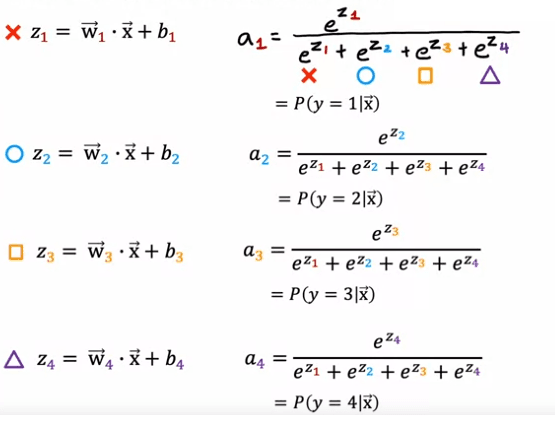
The formula for softmax regression is as follows: a1 = e^z1/ (e^z1 + e^z2 + e^z3 + e^z4), and this will be interpreted as the algorithm's estimate of the chance of y being equal to 1 given the input features x. Similarly, a2 = e^z2 / (e^z1 + e^z2 + e^z3 + e^z4) will be the estimate of the chance of y being equal to 2 given the input features x. Similarly, a3 and a4 will be calculated as e^z3 / (e^z1 + e^z2 + e^z3 + e^z4) and e^z4 / (e^z1 + e^z2 + e^z3 + e^z4) respectively.
It is important to note that the sum of all a1, a2, a3, a4 will be equal to 1, as they represent the probabilities of y taking on the values 1, 2, 3 or 4 respectively.
In the general case, where y can take on n possible values, the formulas for softmax regression can be expressed as: ai = e^zi / (e^z1 + e^z2 + ... + e^zn) for i = 1, 2, 3, ..., n.

In summary, softmax regression is a multiclass classification algorithm that estimates the probability of the output variable y taking on different values given the input features x. It has parameters w1 through wn and b1 through bn, and if appropriate choices for these parameters can be learned, it can predict the chances of y being 1, 2, 3, ..., n given a set of input features x.
How to apply it
In order to build a Neural Network that can carry out multi class classification, we're going to take the Softmax regression model and put it into essentially the output layer of a Neural Network.
Previously, when we were doing handwritten digit recognition with just two classes, we used a Neural Network with this architecture. If we now want to do handwritten digit classification with 10 classes, all the digits from zero to nine, then we're going to change this neural Network to have 10 output units. And this new output layer will be a Softmax output layer. So sometimes we'll say this Neural Network has a Softmax output or that this upper layer is a Softmax layer.
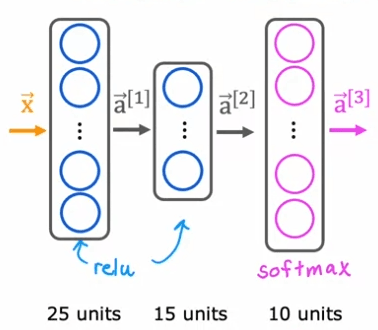
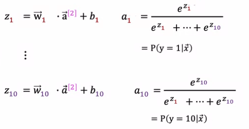
The way forward propagation works in this Neural Network is given an input X, A1 gets computed exactly the same as before. And then A2, the activations for the second hidden layer also get computed exactly the same as before. And we now have to compute the activations for this output layer, that is a3. If you have 10 output classes, we will compute Z1, Z2 through Z10 using these expressions. So this is actually very similar to what we had previously for the formula you're using to compute Z. Z1 is W1.product with a2, the activations from the previous layer plus b1 and so on for Z1 through Z10. Then a1 is equal to e to the Z1 divided by e to the Z1 plus up to e to the Z10. And that's our estimate of the chance that y is equal to 1. And similarly for a2 and similarly all the way up to a10.
It is important to note that the sum of all a1, a2, a3, a4 will be equal to 1, as they represent the probabilities of y taking on the values 1, 2, 3 or 4 respectively.
The Softmax layer will sometimes also called the Softmax activation function, it is a little bit unusual in one respect compared to the other activation functions we've seen so far, like sigma, radial and linear, which is that when we're looking at sigmoid or value or linear activation functions, a1 was a function of Z1 and a2 was a function of Z2 and only Z2. In other words, to obtain the activation values, we could apply the activation function g be it sigmoid or rarely or something else element wise to Z1 and Z2 and so on to get a1 and a2 and a3 and a4. But with the Softmax activation function, notice that a1 is a function of Z1 and Z2 and Z3 all the way up to Z10. So each of these activation values, it depends on all of the values of Z.
Finally, let's look at how you would implement this in TensorFlow. Similar as before there are three steps to specifying and training the model. The first step is to tell TensorFlow to sequentially string together three layers. The first layer is this 25 units with relu activation function. The second layer is 15 units of relu activation function. And then the third layer, because there are now 10 output units, you want to output a1 through a10, so there are now 10 output units. And we'll tell TensorFlow to use the Softmax activation function.
 model = Sequential(
    [
        Dense(25, activation='relu', name = 'layer1'),
        Dense(15, activation='relu', name = 'layer2'),
        Dense(10, activation='softmax', name = 'layer3')
    ], name = "my_model"
)
And the cost function will be the cross-entropy loss. The second step is to train the model using the training data, and the final step is to evaluate the model's performance on the test data.
 model.compile(
    loss=SparseCategoricalCrossentropy())
)

model.fit(X,Y,epochs=100)
In summary, to build a Neural Network that can carry out multi class classification, we can take the Softmax regression model and put it into the output layer of a Neural Network. The forward propagation works by computing the activations for the output layer using the Softmax activation function. This gives us estimates of the probability of the output variable y taking on different values given the input features x. The Softmax layer is unique in that each activation value depends on all the values of Z. It can be implemented in TensorFlow by specifying and training the model using the appropriate layers and activation functions.
Improved the softmax function
In this section, we will explore the importance of numerical stability when implementing machine learning algorithms, specifically in the context of logistic and softmax regression.
First, let's consider an example of how numerical round-off errors can occur in computations. When computing the value 2/10,000, we have two options:
- Option 1: set x = 2/10,000.
- Option 2: set x = (1 + 1/10,000) -(1 -1/10,000).
When we print out the results of these options, we can see that the second option has a small amount of round-off error. This is because the computer has a limited amount of memory to store each number, known as a floating-point number. Depending on how we decide to compute the value 2/10,000, the result can have more or less numerical round-off error.
Now let's examine how these ideas apply to logistic regression. In logistic regression, we compute the loss function for a given example by first computing the output activation, a, which is g(z) or 1/(1 + e ^-z). Then we compute the loss using this expression.
In the traditional implementation, we compute a as an intermediate value and then use it to compute the loss. However, it turns out that by specifying the loss function directly (i.e. without computing a as an intermediate value), TensorFlow can rearrange terms and compute the loss function in a more numerically accurate way. This is achieved by setting the output layer to use a linear activation function and including both the activation function and the cross-entropy loss in the specification of the loss function. The code for this implementation is shown below:
model.compile(loss=SparseCategoricalCrossEntropy(from_logits=True))
While this implementation may be less legible, it results in less numerical round-off error. In the case of logistic regression, either of these implementations works okay, but numerical round-off errors can become worse when it comes to softmax.
To improve the accuracy of our softmax implementation, we can use the same approach as we did with logistic regression. Instead of computing the activations as separate intermediate terms, we can specify the loss function directly as it relates to the output values.
This gives TensorFlow the flexibility to rearrange terms and compute the loss function in a more numerically accurate way. The code for this is shown as follows: in the output layer, we set it to use a linear activation function and the computation of the loss is then captured in the loss function, where we have the "from_logits=True" parameter. This implementation may be less legible, but it results in less numerical round-off error and should be used for more accurate computations within TensorFlow.
It's important to note that by using this approach, we've changed the neural network to use a linear activation function rather than a softmax activation function. This means that the neural network's final layer no longer outputs probabilities, but instead outputs z_1 through z_10. In the case of logistic regression, we also have to change the code to take the output value and map it through the logistic function in order to get the probability.
Multi-label classification problem
When it comes to building a neural network for image classification, there are two main types of problems to consider: multi-class classification and multi-label classification.
In a multi-class classification problem, there is a single label associated with each input image.
For example, in a handwritten digit classification problem, the target label (Y) is a single number, even if that number can take on 10 different possible values.
On the other hand, in a multi-label classification problem, there can be multiple labels associated with each input image.
For example, in a self-driving car application, given a picture of what's in front of the car, we may want to ask questions like, "Is there a car or at least one car? Is there a bus? Is there a pedestrian or are there any pedestrians?" In this case, the target label (Y) is a vector of three numbers, corresponding to whether or not there are any cars, buses, or pedestrians in the image.
One way to build a neural network for multi-label classification is to treat it as three separate machine learning problems. For example, we could build one neural network to decide, are there any cars? The second one to detect buses and the third one to detect pedestrians. However, another way to do this is to train a single neural network to simultaneously detect all three of cars, buses, and pedestrians.
To achieve this, our neural network architecture would have an input layer, followed by one or more hidden layers, and a final output layer with multiple nodes. Because we are solving three binary classification problems, we can use a sigmoid activation function for each of these output nodes. The final output of the network would be a vector of three numbers.
Adam algorithm
Adam stands for Adaptive Moment Estimation, and it is a popular optimization algorithm used in deep learning. Unlike traditional optimization algorithms that use a single global learning rate, Adam uses different learning rates for every single parameter of the model. This allows the algorithm to adapt the learning rate to the specific behavior of each parameter.
The intuition behind the Adam algorithm is that if a parameter seems to keep moving in roughly the same direction, the learning rate for that parameter should be increased to go faster in that direction. Conversely, if a parameter keeps oscillating back and forth, the learning rate for that parameter should be reduced to prevent it from oscillating.
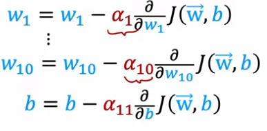
The details of how Adam adapts the learning rate for each parameter are a bit complicated, but it is implemented in code by using the tf.keras.optimizers.Adam optimizer. The Adam optimization algorithm needs a default initial learning rate, and in this example, it is set to 10^-3. However, when using the Adam algorithm in practice, it is worth trying different values for the initial learning rate to see which one gives the best performance.
Compared to the original gradient descent algorithm, the Adam algorithm is more robust to the exact choice of learning rate and typically works much faster. It has become a de facto standard in how practitioners train their neural networks, and if you are trying to decide which optimization algorithm to use, a safe choice would be to use the Adam optimization algorithm.
 import tensorflow as tf

# Define the model
model = tf.keras.Sequential()
model.add(tf.keras.layers.Dense(10, input_shape=(784,)))
model.add(tf.keras.layers.Activation('relu'))
model.add(tf.keras.layers.Dense(10))
model.add(tf.keras.layers.Activation('softmax'))

# Compile the model
model.compile(optimizer=tf.keras.optimizers.Adam(learning_rate=0.001),
              loss='categorical_crossentropy',
              metrics=['accuracy'])

# Train the model
model.fit(x_train, y_train, epochs=10, batch_size=32)
Convolutional layer
In this article, we will take a look at a different type of layer in neural networks called a convolutional layer. This type of layer is used in some applications because it can speed up computation and make a neural network require less training data or be less prone to overfitting.
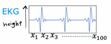
A convolutional layer is a layer where each neuron only looks at a region of the input image, rather than all of the pixels. This can be illustrated with an example of classifying EKG signals. In this example, the first hidden unit in a convolutional layer would only look at a small window of the EKG signal, such as X1 through X20. The second hidden unit would look at a different window, such as X11 through X30, and so on. This is a convolutional layer because these units in this layer look at only a limited window of the input.
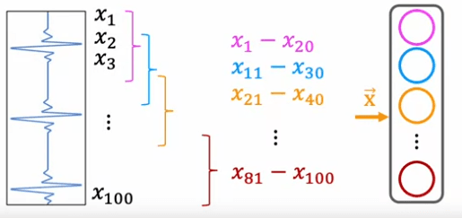
It is important to note that the next layer can also be a convolutional layer. In the second hidden layer, the first unit may look at just the first 5 activations from the previous layer, the second unit may look at just another five numbers, and the third and final hidden unit in this layer will only look at a certain set of activations. Finally, these activations are input to a sigmoid unit that does look at all of these values in order to make a binary classification regarding the presence or absence of heart disease.
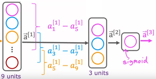
In this example, the neural network has a first hidden layer that is a convolutional layer, a second hidden layer that is also a convolutional layer, and an output layer that is a sigmoid layer. There are many architectural choices when using convolutional layers, such as how big the window of inputs that a single neuron should look at and how many neurons the layer should have. By choosing these architectural parameters effectively, you can build new versions of neural networks that can be even more effective than the dense layer for some applications.
To summarize, convolutional layers and convolutional neural networks are a different type of layer
Evaluating the model
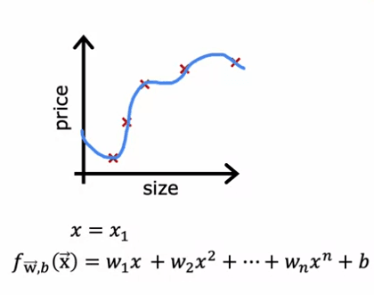
Learning to predict housing prices as a function of the size can be a difficult task. To help with this, a model can be trained to predict housing prices as a function of the size x. One example of this is a fourth order polynomial, which includes features such as:
| x1 | Size |
|---|---|
| x2 | Numbers of bedrooms |
| x3 | Numbers of floors |
| x4 | Age of home in years |
This model may fit the training data well, but it may not generalize well to new examples that are not in the training set.
When predicting prices, it can be difficult to tell if a model is performing well, especially when there are more than one or two features. One technique that can be used to evaluate a model's performance is to split the training set into two subsets: a training set and a test set. The model's parameters can be trained on the training set and then tested on the test set.
For example, if a dataset has ten examples:
| Size | Prices |
|---|---|
| 2104 | 400 |
| 1600 | 330 |
| 2400 | 369 |
| 1416 | 232 |
| 3000 | 540 |
| 1985 | 300 |
| 1534 | 315 |
| 1427 | 199 |
| 1380 | 212 |
| 1494 | 243 |
It can be split into a training set of 70% of the data and a test set of 30% of the data. In this example, the training set would have seven examples and the test set would have three examples.
mtrain = no.training examples = 7 mtest = test set = 3
To train a model using linear regression with a squared error cost, the parameters can be fit by minimizing the cost function, which includes a regularization term. The model's performance can then be evaluated by computing the average error on the test set, also known as J test of w,b. This is done by computing the squared error on each test example and averaging it over the number of test examples.
When it comes to evaluating the performance of machine learning algorithms, it's important to consider both the training error and the test error. The training error gives us an idea of how well the model is fitting the data it's been trained on, but it doesn't give us an indication of how well the model will perform on new, unseen data. This is where the test error comes in.
One way to define the training error and test error is by using the concepts of J train and J test. J train is defined as the average over the training set of the squared error term, without the regularization term. In other words, it measures the average error the model makes on the training data. On the other hand, J test is defined as the average over the test set (examples not used in training) of the error term, without the regularization term. It measures the average error the model makes on the test data.
When we're dealing with regression problems, a low J train value is generally a good sign. It means that the model is performing well on the training data, and that the average error on training examples is zero or very close to zero. However, if J test is high, it's an indication that the model is not generalizing well to new examples or data points not in the training set. This means that even though the model is performing well on the training data, it's not likely to perform well on new, unseen data.
In classification problems, J train and J test can be defined in a slightly different way. Instead of using the logistic loss to compute the test error and the training error, a more commonly used method is to measure the fraction of the test set and training set that the algorithm has misclassified. For example, in a classification problem of handwritten digits 0 or 1, J test would be the fraction of the test set where 0 was classified as 1 or 1 was classified as 0. Similarly, J train would be the fraction of the training set that has been misclassified.
It's important to note that the test error rate is always higher than the training error rate. That's because the model is trained to fit the training data as well as possible, and it will always perform better on the data it's been trained on than on new, unseen data.
In conclusion, by splitting a dataset into a training set and test set, and computing both J tests and J train, we can systematically evaluate how well the learning algorithm is doing. This procedure allows for measuring the performance on the test set and the training set, and can be used as a step in automatically choosing the appropriate model for a given machine learning application. It is a crucial step in evaluating and improving the performance of machine learning models.
Model selection
It's important to note that the training error of a machine learning model is not always a good indicator of how well it will perform on new, unseen examples. In this article, we will explore how using a test set can help us choose a model for a given machine learning application.
Consider a scenario where we are trying to fit a function to predict housing prices using a linear model, such as a first-order polynomial. We fit this model to our training set, and obtain parameters w and b. We can then compute the test set error, J_test, to estimate how well the model will generalize to new data.

Now, let's say we also consider fitting a second-order polynomial and a third-order polynomial, and continue this process up to a tenth-order polynomial. We will obtain J_test for each of these models, giving us a sense of how well each one is performing. One procedure we could try is to look at all of these J_tests, and see which one gives the lowest value. For example, if we find that J_test for the fifth-order polynomial (d=5) turns out to be the lowest, we might decide to choose that model for our application.
the cross-validation
However, this procedure is flawed. Using the test set to choose the parameter d (in this case, the degree of the polynomial) can result in an overly optimistic estimate of the generalization error. To avoid this issue, we can modify the training and testing procedure by splitting our data into three subsets: the training set, the cross-validation set, and the test set.
| Size | Prices |
|---|---|
| 2104 | 400 |
| 1600 | 330 |
| 2400 | 369 |
| 1416 | 232 |
| 3000 | 540 |
| 1985 | 300 |
| 1534 | 315 |
| 1427 | 199 |
| 1380 | 212 |
| 1494 | 243 |
For example, we might use 60% of our data for the training set, 20% for the cross-validation set, and the remaining 20% for the test set. We can then use the cross-validation set to choose the best model, and report the test set error as an estimate of the model's performance on new data. By using this modified procedure, we can avoid the issue of choosing a model that may not perform well on new data.
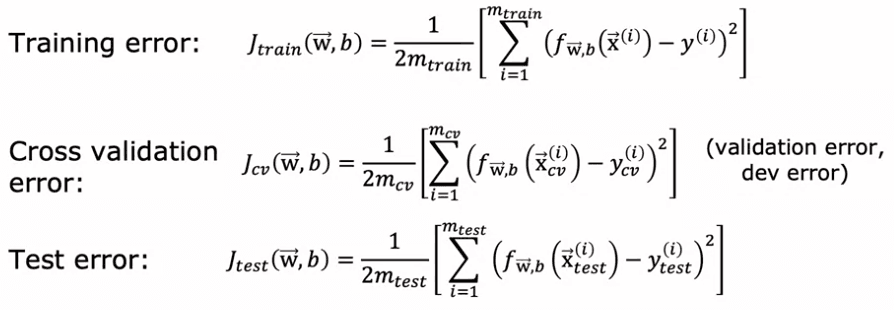
The way we'll modify the procedure is instead of splitting your data into just two subsets, the training set and the test set, we're going to split your data into three different subsets, which we're going to call the training set, the cross-validation set, and then also the test set. Using our example from before of these 10 training examples, we might split it into putting 60 percent of the data into the training set and so the notation we'll use for the training set portion will be the same as before, except that now M train, the number of training examples will be six and we might put 20 percent of the data into the cross-validation set and a notation I'm going to use is x_cv of one, y_cv of one for the first cross-validation example. So cv stands for cross-validation, all the way down to x_cv of m_cv and y_cv of m_cv. Where here, m_cv equals 2 in this example, is the number of cross-validation examples. Then finally we have the test set same as before, so x1 through x m tests and y1 through y m tests. The test set is going to be the same size as the cross-validation set, so 20 percent of the total data.
Now, with this new three-way split of the data, we can use the training set to fit our model and the cross-validation set to choose the best model. In other words, we can use the cross-validation set to choose the best value of d, the degree of the polynomial. We can try fitting a first-order polynomial and get J_cv^1, then try fitting a second-order polynomial and get J_cv^2, and so on, up to a tenth-order polynomial, and get J_cv^10. From these values, we can choose the value of d that gives us the lowest J_cv. Let's say we choose d=5, then we can use the test set to get an estimate of the generalization error, J_test^5. This estimate of the generalization error is less likely to be overly optimistic because we did not use the test set to choose the value of d.
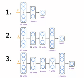
In summary, using a three-way split of the data with a training set, a cross-validation set, and a test set allows us to choose the best model without biasing our estimate of the generalization error. The training set is used to fit the model, the cross-validation set is used to choose the best model, and the test set is used to estimate the generalization error. This is a more robust way to carry out model selection for machine learning applications.

 English
